Usage

Configuration

Various parameters are controlled by values given in a text-based configuration file. The user can choose any filename for this configuration file. Example parameters for running PyRate with GAMMA-format interferograms are contained in the example configuration file PyRate/input_parameters.conf.

Workflow

File Discovery

To allow flexibility in the file types that can be processed, PyRate requires file lists to be provided. This allows PyRate to identify files of each type without relying on file extensions. The file path to these lists are provided under ifgfilelist, hdrfilelist, cohfilelist and basefilelist keywords in the configuration file. These lists can be created manually or generated using the script list_creator.sh located in the utils folder. This script may need to be slightly modified depending on the output paths of your input data.

Note

• Filenames should be provided in these lists with their absolute system path, with each name on a separate line.

• Filenames should only have a single period (“.”) delimiting the file extension. Multiple periods in a filename will raise an error during runtime.

The ifgfilelist gives the list of interferograms to be processed. Example of an interferogram file list for GAMMA flat-binary files:

/absolute/path/to/20150702-20150920.unw
/absolute/path/to/20151219-20160109.unw
/absolute/path/to/20160202-20160415.unw

Note

• Interferogram filenames must contain a pair of date epochs. Any naming convention is appropriate as long as an epoch pair of format YYYYMMDD-YYYYMMDD or YYMMDD-YYMMDD exists in the filename.

The hdrfilelist gives the list of GAMMA Multi-Look Intensity (MLI) header text files. Example of a GAMMA MLI header file list:

/absolute/path/to/20150702_mli.par
/absolute/path/to/20150920_mli.par
/absolute/path/to/20151219_mli.par
/absolute/path/to/20160109_mli.par
/absolute/path/to/20160202_mli.par
/absolute/path/to/20160415_mli.par

Note

• MLI header filenames must contain a single date epoch in the format YYYYMMDD or YYMMDD.

• GAMMA Single-Look Complex (SLC) header files could be used instead, but the geometry calculations in prepifg will not work, and subsequently the DEM Error correction step in correct will not work. Both require parameters valid for the multi-looked radar-coded interferograms.

The cohfilelist is an optional list which contains the pool of all available coherence files to be used for optional coherence masking. Example of a coherence file list for GAMMA flat-binary files:

/absolute/path/to/20150702-20150920.coh
/absolute/path/to/20151219-20160109.coh
/absolute/path/to/20160202-20160415.coh

Note

• Like interferograms, coherence filenames must contain a pair of epochs. The epoch pair must be in the format YYYYMMDD-YYYYMMDD or YYMMDD-YYMMDD. Otherwise, any naming convention is appropriate.

The basefilelist is an optional list which contains the pool of all available GAMMA baseline vector files. These are only needed if the user wants to use the DEM error correction functionality. Example of a baseline file list for GAMMA baseline vector files:

/absolute/path/to/20150702-20150920_base.par
/absolute/path/to/20151219-20160109_base.par
/absolute/path/to/20160202-20160415_base.par

The date epochs in filenames are used to match the corresponding MLI header or coherence files to each interferogram. It is recommended to provide a complete list of available headers/coherence/baseline files for a stack in their respective lists, since only the necessary files will be used. This allows you to process a subset of interferograms by removing entries in ifgfilelist without needing to modify all four lists.

PyRate Workflow

After Installation, an executable program pyrate is created in the system path:

   >> pyrate --help
   usage: pyrate [-h] [-v {DEBUG,INFO,WARNING,ERROR}]
                 {conv2tif,prepifg,correct,timeseries,stack,merge,workflow} ...

   PyRate workflow:

       Step 1: conv2tif
       Step 2: prepifg
       Step 3: correct
       Step 4: timeseries
       Step 5: stack
       Step 6: merge

   Refer to https://geoscienceaustralia.github.io/PyRate/usage.html for
   more details.

   positional arguments:
     {conv2tif,prepifg,correct,timeseries,stack,merge,workflow}
       conv2tif            <Optional> Convert interferograms to geotiff.
       prepifg             Perform multilooking, cropping and coherence masking to interferogram geotiffs.
       correct             Calculate and apply corrections to interferogram phase data.
       timeseries          <Optional> Timeseries inversion of interferogram phase data.
       stack               <Optional> Stacking of interferogram phase data.
       merge               Reassemble computed tiles and save as geotiffs.
       workflow            <Optional> Sequentially run all the PyRate processing steps.

   optional arguments:
     -h, --help            show this help message and exit
     -v {DEBUG,INFO,WARNING,ERROR}, --verbosity {DEBUG,INFO,WARNING,ERROR}
                           Increase output verbosity

.. note::

   - If running on NCI, be sure to first load the correct modules and virtual environment:
     ``source ~/PyRate/scripts/nci_load_modules.sh``

The pyrate program has six command line options corresponding to different steps in the PyRate workflow:

1. conv2tif (optional)

2. prepifg

3. correct

4. timeseries (optional)

5. stack (optional)

6. merge

Not all steps are required as indicated above. A seventh option, workflow, is available that will run all six of the above steps in the order shown.

Command line arguments for each step can be found using (e.g. for conv2tif):

>> pyrate conv2tif --help
usage: pyrate conv2tif [-h] -f CONFIG_FILE

optional arguments:
  -h, --help            show this help message and exit
  -f CONFIG_FILE, --config_file CONFIG_FILE
                        Pass configuration file

Each step can be run on the command line in one of the following two ways (e.g. for conv2tif):

>> pyrate conv2tif -f /path/to/config_file

or:

>> python3 pyrate/main.py conv2tif -f /path/to/config_file

In the following sub-sections we describe each of the available steps.

conv2tif: Converting flat-binary files to Geotiff format

Before PyRate can process interferograms that are in flat-binary file format, they need to be converted into geotiff format using the optional conv2tif step.

Note

• Users of the GAMMA software can skip the conv2tif step if they have generated geotiffs using the GAMMA program data2geotiff, which is included in all GAMMA software distributions.

• In this case, ifgfilelist and cohfilelist would contain the absolute paths to these geotiff files. Even when using geotiff files, the MLI header files are still required by prepifg.

• If a DEM is to be processed by prepifg, it’s file format should match the input interferograms (e.g. geotiff or flat-binary files).

Upon completion of conv2tif geotiff formatted copies of the input files will be placed in the <outdir> directory defined in the configuration file.

Note

• conv2tif will not perform the conversion if geotiffs for the provided input files already exist.

prepifg: Preparing input interferograms

prepifg is the second step of PyRate, which applys optional multi-looking (sub-sampling), cropping and coherence masking operations to the geotiff-format input interferograms. This is a required step, which formats the input data in a way expected by the rest of the PyRate workflow.

Coherence masking

prepifg will perform optional coherence masking on the interferograms before multi-looking and cropping is performed. This requires corresponding coherence images for each interferogram. The purpose of coherence masking is to remove poor quality phase observations and leave a set of high-quality pixels for analysis.

Coherence masking is enabled by setting cohmask: 1 in the configuration file. A threshold, cohthresh needs to be provided. Pixels with coherence values below cohthresh will be set to Not-a-Number (NaN).

Note

• The number of pixels with numeric phase values (i.e. pixels not equal to NaN) will be different in each interferogram after coherence masking.

The available coherence files need to be specified in a list file as described above and defined in the cohfilelist parameter.

Note

• Multi-looked and cropped versions of those coherence images found that match the epochs of the input interferograms will be saved to disk in geotiff format, even if coherence masking is not applied (i.e. cohmask: 0).

• Additionally, the mean, median and standard deviation of the coherence for each pixel is calculated and saved as part of prepifg.

• All coherence files are saved to the <outdir>\coherence_dir directory.

Multi-looking

The prepifg step will perform optional multi-looking (image sub-sampling) of the input interferograms in geotiff format. The purpose of multi-looking is twofold:

• Reduce the spatial resolution of the interferograms in order to improve the computational efficiency of PyRate analysis.

• Reduce the general phase noise in the interferograms in order to enhance the signal-to-noise ratio in the output products.

To multi-look, set ifglksx and ifglksy to an integer subsampling factor greater than one in the x (easting) and y (northing) dimensions respectively. Separate parameters for x and y gives flexibility for users in case they want to achieve different spatial resolution in each dimension.

Note

• For example, a value of 2 will reduce the resolution by half. A value of 1 will keep the resolution the same as the input interferograms (i.e. no multi-looking).

• It is recommended to try a large multi-look factor to start with (e.g. 10 or greater), and subsequently reduce the multi-looking factor once the user has experience with processing a particular dataset.

Cropping

The prepifg step will perform optional spatial cropping of the input interferograms. This is useful if you are focussing on a specific area of interest within the full extent of the input interferograms. The advantage of cropping is that PyRate analysis will be computationally more efficient.

To crop, set ifgcropopt to 3 and provide the geographic latitude and longitude bounds in the ifgxfirst (west), ifgxlast (east), ifgyfirst (north), and ifgylast (south) parameters.

Geometry calculations

During the prepifg step, the radar viewing geometry for every pixel is calculated using metadata from the GAMMA MLI parameter files.

Note

• Geometry calculations are only implemented for GAMMA format input data.

The output arrays are saved to <outdir>/geometry_dir and contain as follows:

• rdc_azimuth.tif: azimuth coordinate in range-doppler system;

• rdc_range.tif: range coordinate in range-doppler system;

• look_angle.tif: look angle (vector between line-of-sight and satellite nadir);

• incidence_angle.tif: incidence angle (vector between line-of-sight and vector perpendicular to local ground surface);

• azimuth_angle.tif: azimuth angle (projection of line-of-sight on the surface);

• range_dist.tif: satellite to ground range distance;

• dem.tif: digital elevation model.

Upon completion, prepifg will save a new set of interferogram files in the <outdir>\interferogram_dir (*_ifg.tif). If provided as input, coherence files will be saved to <outdir>\coherence_dir (*_coh.tif).

correct: Compute and apply interferometric phase corrections

correct is the third step in the PyRate processing workflow. This step will perform a series of optional corrections to the interferogram phase data and apply a number of prepatory steps required prior to data inversion.

The sub-steps are performed in the following default order:

• Search for a suitable reference pixel;

• Residual Orbit error correction (optional, controlled by orbfit parameter);

• Correction of reference phase in interferograms;

• Residual DEM error correction (optional, controlled by demerror parameter);

• Unwrapping error detection and masking (optional, controlled by phase_closure parameter);

• Minimum Spanning Tree matrix formation;

• Spatio-temporal filtering of the interferograms ((optional, controlled by apsest parameter);

• Calculation of interferogram spatial covariance functions;

• Assembly of the variance-covariance matrix.

This default order of steps can be modified by the user by copying the following code block in to the configuration file and switching the order of steps as required:

[correct]
steps =
    orbfit
    refphase
    demerror
    phase_closure
    mst
    apscorrect
    maxvar

The corrected interferogram phase is saved to copies of the prepifg interferograms in the directory <outdir>/temp_mlooked_dir/ (the original output from prepifg is retained as a read-only interferogram dataset in the <outdir>/interferogram_dir). Additionally, copies of the phase corrections subtracted from interferograms are saved to disk as numpy array files (*.npy) for use in post-processing. These can be found in labelled sub-directories in the <outdir>.

timeseries: Compute the displacement time series

timeseries is the optional fourth step in the PyRate processing workflow. This step will perform a time series inversion to derive the cumulative displacement time series from the stack of corrected interferograms. The cumulative displacement time series (tscuml*) is saved by default. Users can optionally save the incremental displacement time series (tsincr*) by setting parameter savetsincr: 1.

A linear regression of the cumulative displacement time series is also computed as part of the timeseries step. The resulting linear rate (velocity), standard error, R-squared and y-intercept terms are all saved to disk.

stack: Compute the average velocity via stacking

stack is the optional fifth step in the PyRate processing workflow. This step will perform an iterative stacking of the phase data to derive a robust velocity estimate for each pixel in the interferograms. The velocity from stacking (stack_rate*) is saved by default.

Note

• Both timeseries and stack are optional and independent steps that can be computed in either order.

merge: Reassemble the tiles

merge is the sixth and final step of the PyRate workflow, which produces geotiff files containing the final time series, linear rate and stacking products. merge will also re-assemble tiles that were generated during the previous steps. Tiling is discussed in the Parallel Processing section below.

The final outputs contain signals in the line-of-sight (LOS) of the satellite. Using the los_projection option, the user can project those signals to either the pseudo-vertical (set to 1) or pseudo-horizontal (set to 2). This projection makes use of the per-pixel incidence angle image generated during prepifg.

Note

• Users should be aware that the pseudo-vertical and pseudo-horizontal signal projections do not necessarily represent the true vertical or horizontal ground movement signal. The true signals cannot be recovered with InSAR data from a single LOS viewing geometry.

• If the user has InSAR data from multiple viewing geometries (e.g. from both ascending and descending orbits), signal decomposition can be carried out after PyRate analysis as a post-processing step.

If necessary, the user can switch the polarity of the final output products by setting signal_polarity: -1.

The error products produced by PyRate can be scaled by n-sigma using the parameter velerror_nsig.

After running the merge step, several geotiff products will appear in the <outdir>/velocity_dir and <outdir>/timeseries_dir directories.

workflow: Run the full PyRate workflow

workflow is an additional option that will run all the above six steps in order as a single job. This could be useful for batch processing runs.

Input Files

PyRate currently supports input files generated by the GAMMA, ROI_PAC and SNAP interferometry softwares. PyRate will determine the input format from the processor: parameter in the configuration file (0: ROI_PAC; 1: GAMMA (and SNAP)).

GAMMA

Each GAMMA geocoded unwrapped interferogram requires three header files to extract metadata required for data formatting: a geocoded DEM header file (demHeaderFile keyword in the configuration file) and the relevant MLI image header files (*mli.par) found in the hdrfilelist. The header files for the first and second MLI images used in the formation of a particular interferogram are found automatically by date-string pattern matching based on date epochs given in the filenames. A DEM with matching size and geometry to the interferograms can also be processed. The DEM absolute path and filename are set with the demfile parameter.

SNAP

The European Space Agency SNAP software has supported PyRate since version 8.0.0. Users can convert their output data in to GAMMA format by using the “PyRate export” function in SNAP. Then users should follow the PyRate instructions for GAMMA-formatted data.

Note

• The capability to generate SBAS interferogram networks that are needed for time series analysis of large InSAR stacks in PyRate is planned for a future version of SNAP.

ROI_PAC

Each ROI_PAC geocoded unwrapped interferogram requires its own header/resource file (*.rsc). These header files need to be listed in the defined hdrfilelist. In addition, the geocoded DEM header file is required and its path and name are specified in the config file under demHeaderFile. The geographic projection in the parameter DATUM: is extracted from the DEM header file. A DEM with matching size and geometry to the interferograms can also be processed. The DEM absolute path and filename are set with the demfile parameter.

Note

• Support and development of ROI_PAC has been discontinued.

• ROI_PAC support in PyRate will be deprecated in a future release.

Parallel Processing

By their very nature, interferograms are large files. This is particularly the case for Sentinel-1, which has an image swath of 250 km and a pixel resolution on the order of tens of metres in IW-mode. Consequently, InSAR processing can be computationally expensive and time consuming. It therefore makes sense to parallelise processing operations wherever possible.

PyRate can be run in parallel using standard multi-threading simply by turning parallel: 1 in the configuration file to take advantage of multiple cores on a single machine. The parameter processes sets the number of threads.

Alternatively, PyRate can be parallelised on a system with an installed MPI library by using mpirun:

# Modify '-n' based on the number of processors available.
mpirun -n 4 pyrate conv2tif -f path/to/config_file
mpirun -n 4 pyrate prepifg -f path/to/config_file
mpirun -n 4 pyrate correct -f path/to/config_file
mpirun -n 4 pyrate timeseries -f input_parameters.conf
mpirun -n 4 pyrate stack -f input_parameters.conf
mpirun -n 4 pyrate merge -f path/to/config_file

Note

• In the case that PyRate is run using mpirun, standard multi-threading is automatically disabled (i.e. equivalent to setting parallel: 0).

During conv2tif and prepifg, parallelism is achieved by sending sub-lists of input files to each process. Parallelism in the correct, timeseries and stack steps is achieved by splitting the images in to a grid of tiles, where the number of tiles equals the number of processes passed with the -n argument to mpirun, or the processes parameter for multi-threading. The number of tiles in x and y dimension are automatically calculated by PyRate, ensuring a roughly equivalent number in both dimensions. One of the functions of the merge step is to reassemble these tiles in to the full image for each output product.

Results Visualisation

Several plotting scripts are included in the utils/ directory to help the user visually inspect the output products of PyRate:

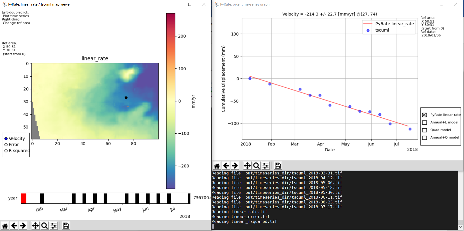
• make_tscuml_animation.py: Make an animated gif from cumulative time series data;

• plot_linear_rate_profile.py: Plot a profile through a linear rate map;

• plot_time_series.py: Map and graph view of cumulative time series data;

• plot_correction_files.py: Before and after viewing of interferogram corrections;

• plot_sbas_network.py: Baseline-time plot for the interferogram network.

Example usage of plot_time_series.py with the included test data:

cd PyRate
source ~/PyRateVenv/bin/activate
pyrate workflow -f input_parameters.conf
pip install -r requirements-plot.txt
python3 utils/plot_time_series.py out/