2 Model Concepts
SIRA provides a modelling framework and software tools for assessing impact of natural hazards on infrastructure systems. Infrastructure systems, within this framework, refer to facilities and networks that provide essential utility services for communities, regions and/or a country. This will include electricity generation and transmission, water and wastewater treatment and reticulation, and transport networks. It excludes standalone high-value buildings and manufacturing plants. The SIRA project also deliberately eschews an exclusive focus on “critical” infrastructure, as that invites unnecessary debates on criteria of criticality and jurisdiction for that class of assets.
2.1 The ‘System’ Model
A system, according to the Merriam-Webster dictionary, is:
“a regularly interacting or interdependent group of items forming a unified whole.”
The International Council on Systems Engineering (INCOSE) has the following simple definition for a system on its website:
“A system is a set of elements that work together to produce results that the individual elements couldn’t achieve alone.”
INCOSE also provides a more specific definition of a ‘complex system’ that emphasises the non-trivial relationships between cause and effect, associated its ‘emergent’ properties [7]:
“A complex system is a system in which there are non-trivial relationships between cause and effect: each effect may be due to multiple causes; each cause may contribute to multiple effects; causes and effects may be related as feedback loops, both positive and negative; and cause-effect chains are cyclic and highly entangled rather than linear and separable.”
This definition of a complex system is particularly relevant to the SIRA modelling framework, as it captures the essence of the interdependencies and interactions that characterise infrastructure systems. The SIRA simulation approach is designed to account for these complexities and provide insights into how disruptions from hazards can lead to potentially unpredictable behaviours and propagate through the system, affecting its overall functionality.
The specific meaning of a system and its boundaries depend on the context, and it is important to understand how this term is used within the SIRA modelling methodology. This is clarified in subsequent subsections.
The central idea in the SIRA modelling construct is this: All lifeline infrastructure ‘systems’ within the modelling framework are conceptualised as a network of interconnected nodes.
The nodes or vertices, and connecting edges, have different meaning based on the level of abstraction, which is explained in following subsections.
This modelling approach affords a high degree of flexibility and scalability, making it possible to accommodate multiple sectors and assets of varying scale and complexity.
Furthermore, it allows the user to:
model the effect of impaired or destroyed components on the operational capacity of the overall system;
use graph theory to assess the graduated capacity degradation, and restoration, through modelling flow through the network; and
detect prioritised ‘paths’, or sets of connected components, within the network that need to be repaired or recovered in order to restore the flow through the network which represents the productive capacity of the system.
2.1.1 Infrastructure System Hierarchy
The elements in an infrastructure (or lifeline) system can be conceptualised as being structured in a three-level hierarchy:
Level 1 : Infrastructure Network – This is the top level of interconnected infrastructure systems where infrastructure facilities are connected to form a network or connect to other networks.
Level 2 : Infrastructure Facility – Facilities are geospatially discrete assets that can be linked to a specific physical location and provide a specific service, e.g. a power station or a substation. The concept of facilities used in this framework map closely to the typology of macro-components as defined in the Synerg-G program [8, 9], and align with the definition of systems as defined in [10].
Level 3 : Infrastructure Microcomponent – These are the physical elements that constitute the infrastructure facility, e.g. a transformer or circuit breaker within an electrical substation. This concept of components map closely to the typology of micro-components as defined in the Synerg-G program [8, 9], and align with the definition of subsystems as defined in [10].
This applies to discussions on a complete system that is responsible for delivering some service. This also applies to classification of assets, and how information about those assets are stored and referenced in a database.
2.1.2 Structure of a SIRA Model of a Lifeline Infrastructure
In the context of a specific infrastructure model, developed for hazard impact assessment, the following terms and ideas apply. These are the building blocks of of SIRA model and map to the objects implemented in the simulation code.
The System Model: This defines a logical set of assets that is an abstraction of a real equivalent asset. The usage of the term system in this context is closer to its application in System Engineering, rather than from an IT or software engineering perspective. The System Model defines the boundary of the collection of elements under investigation. It is the collection of nodes and connecting edges that collectively provides a service or generates a type of product. This term can be used to refer to a network or a facility. The context of the simulation will disambiguate its meaning.
Component: It is the high-level element within the network (or graph) that represents the System Model. A collection of interconnected components with specific attributes and roles comprise the System in the context of the simulation model.
The asset being studied will determine what is considered a system or what is considered a component within the context of the simulation.
If the physical system under study is a NETWORK, then the System Model is a Level 1 element, i.e. an Infrastructure Network, and the Components are Level 2 elements, i.e. Infrastructure Facilities.
If the physical system under study is a FACILITY, then the System Model is a Level 2 element, i.e. an Infrastructure Facility, and the Components are Level 3 elements, i.e. Infrastructure Microcomponents.
2.1.3 Classification of Nodes within a Model of an Infrastructure System
For a specific impact assessment project, the Components within the System Model are represented as nodes. Based on their role within the system, these nodes (or components or vertices) are classified in four categories:
Supply nodes: These nodes represent the entry points into the system for required inputs or commodities. As for example, coal and water can be the required ‘commodities’ into a thermal power station. In the case of the substation, required input is electricity from power stations or other substations.
Output nodes: These nodes represent the exit points for the output of the system. They are referred to as sink nodes. For example, in the case of the power station, the output nodes act as dummy loads - representing the energy consumers - connected to each of the step-up transformers. The sum of flow through the network measured at the output nodes represented the effective production (or operational) capacity of the facility.
Dependency nodes: These nodes represent the components that do not directly participate in the production process of the system, or in the handling of system inputs, but are critical for system operations in some other capacity, e.g. system management or monitoring. The control building of a substation is an example of this.
Transhipment nodes: These are nodes that transform, transport, or store system inputs to give effect to processes that produces the outputs required of the system. Majority of the nodes within a system fall into this category.
The component configuration and redundancies are captured as edges connecting the nodes. Constraints on flow through specific paths, or sets of nodes, can be represented as capacities of edges connecting those nodes. Fig. 2.1 illustrates this concept for a thermal power station.
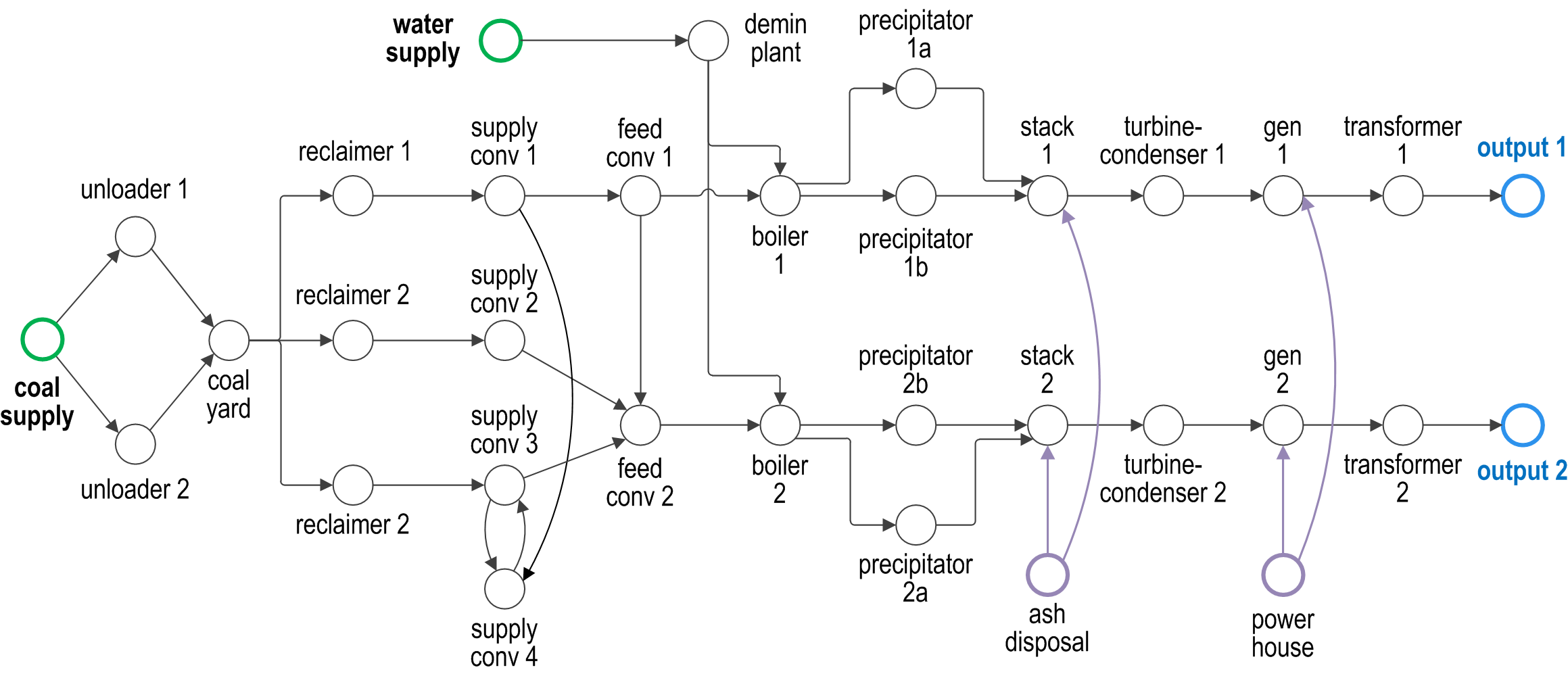
Fig. 2.1 Schematic representation of a coal-fired power station
The ‘edges’, or inter-nodal connections, represent a link or a process for maintaining ‘flow’ of goods or services within the system, and thus their directionality is important. For the power station, the edges are unidirectional, since the inputs flow in one direction starting from the entry point into the system and are progressively transformed through the system to generate energy - the end product. However, a substation is an electrical network where electricity - the system ‘commodity’ - can flow in either direction through an edge (electrical conductor) as dictated by load demands and system constraints. Therefore, most of the edges in the substation are bidirectional, unless specifically constrained.
Connection paths and ‘production capacities’ along those paths within a system are calculated as the maximum flow through those paths. The igraph Python package was used as the network modelling platform to calculate graph metrics for a post-hazard damaged system model.
2.2 System Loss Modelling
For a given level of ground shaking, a set of random samples is generated, and the damage state of each component is calculated for each random sample based on the fragility function of the given component. Given the assessed damage state of all the system components, the system functionality is assessed and system output level calculated. This process is run through a Monte Carlo process for the set of random samples to assess the system response at the selected ground shaking intensity. To obtain a characterisation of the system and develop fragility algorithms for the system (e.g. the power station) the process is repeated for a range of PGA values. This Process is shown in Fig. 2.2.
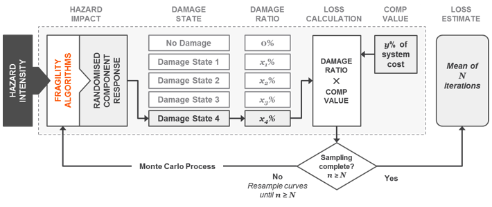
Fig. 2.2 Schematic of process for fragility attribution and loss estimation
Four discrete sequential damage states are used for assessing system fragility, similar to those used in HAZUS (FEMA 2003): DS1 Slight, DS2 Moderate, DS3 Extensive, DS4 Complete. The damage scale used for a power station is based on ranges of economic loss as a percentage of total system value.
The probability of a component exceeding damage state \(ds\) is calculated using the log-normal cumulative distribution function (CDF) as shown in equation below, for a PGA value of \(x\) g:
where, θ = median, and β = logarithmic standard deviation.
For a component in damage state \(ds_i\), the corresponding loss is calculated as:
where,
\(R_{C, ds_i}\) = d is the damage ratio for component C
at damage state \(ds_i\), and
\(CF_C\) = cost of component C as a proportional of total system cost.
2.3 System Restoration Model
The restoration algorithms are defined as normal functions. An approximation of mean restoration time for each component at each damage level is attributed. The structural damage level definitions associated with the damage states are central to establishing a common understanding to facilitate the development of the restoration parameters.
The functionality \(F_C\) of component C at t time units after impact of an earthquake of PGA=x is calculated as a weighted combination of the probability of the components being in each of the S sequential damage states used in the model and the estimated recovery at time t for the components based of the restoration model:
where, \({i}\) is the index of the damage state, \({\{i \in \mathbb{Z} \mid 0 \leq i \leq S\}}\). The ‘None’ damage state is \({i=0}\), and \({i=S}\) is the complete or highest modelled damage state. \(R_i[t]\) is the likely level of restoration of functionality at time \(t\) . Restoration level \(R_i\) can take on any value in the unit interval [0,1].
The simulation of the restoration prognosis is conducted based on a set of inputs and assumptions. The required data inputs to this process are:
The system configuration
The modelled scenario - seismic intensity value
Impact simulation results - system component losses
Restoration priority list - the order at which output lines should be recovered
The process assumes that restoration is undertaken in stages, subject to the level of resources that can be made available and the order of repairs. In regard to this, the concept of ‘Restoration Streams’ is used–the maximum number of components that can be worked on simultaneously. This is effectively a proxy representing the deployment of trained personnel and material for the repair tasks. Additional optional offsets can be factored in to capture specific contexts:
Restoration Offset - this is a time allowance for assessment of damage to the system and for securing the site to assure it is safe for commencement of repairs;
Testing and Commission Interval - this is a time allowance for testing conformity with operational and safety parameters for the system, or a part thereof.
Given a set of restoration parameters and the restoration plan, the consequent restoration time is calculated as follows:
Test if there is any available path between the set of required input nodes (i.e. supply nodes) and the output node assigned the highest priority to meet the demand at that node.
If no functional path is found, then identify the least expensive path(s) that needs to be restored to meet demand at the output node. Within each path, identify the functional status of the nodes (components), and generate a repair list.
Iterate through the ordered output list, repeating steps 1 and 2 above. Update the component repair list and produce a complete prioritised list of components to repair or replace.
Simulate an ordered restoration process based on the above list and user-specified resource constraints. If the process is using x resource constraints, then whenever a component is restored (and the number of unrepaired components is ≥x), the next component is added to the active repair list, so that at any one time x repair tasks are in progress. This process is repeated until all the paths are restored, i.e. until system output capacity is restored to normal levels.
In order to restore full capacity at an output node, it may be necessary to restore more than one path, i.e. connect an output node to multiple input nodes. This can be understood through some simple examples. If the facility in question is a thermal power station, the functioning of the generator depends on both the supply of fuel (as the source of energy to be transformed) and water (for cooling and for steam production to drive the turbines). In case of a substation, a certain output node may have a demand of 300MW, but it might be that there are four incoming lines each bringing in bringing in 100MW of electricity from power plants. In this case, the designated output node must be linked to at least three of the input/supply nodes to meet its demand.
In addition to the core process of approximating restoration time, a routine for simulating component cannibalisation within a facility or system has also been incorporated. Here we use cannibalisation to refer to an exercise whereby an operator may move an undamaged component from a low priority or redundant line to replace a damaged component on a high priority line. This exercise may allow the operator to eliminate the potentially long procurement or transportation time for a replacement unit, and thereby expedite the restoration of the high priority lines.
The outputs from the restoration model are:
A simple Gantt chart with each component needing repair,
Restoration plot for each output line over time and the associated percentage of total system capacity rehabilitated, and
Total restoration time for each output line for a given restoration scheme.