Use of the GUI
This chapter provides an overview of the GUI and instructions on how to run simulations using the GUI.
Structure
The main window is logically divided into five panes by functionality as shown as Fig. 14.
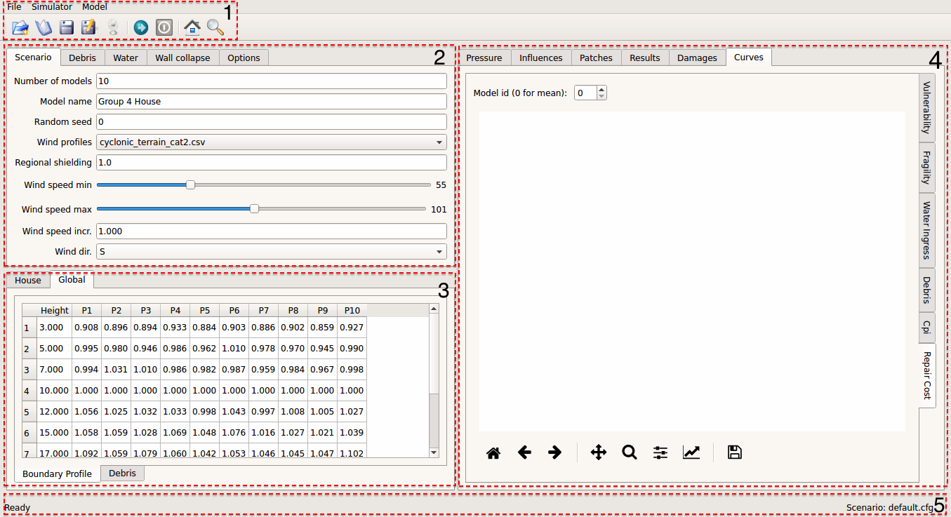
Fig. 14 Program main window consisting of five panes by functionality as shown as dotted box
Pane #1
This pane is located at the top of the main, and consists of tool bar with buttons. The file menu and action corresponding to each of the buttons is set out in the Table 24.
| Button | Menu | Action |
|---|---|---|

|
File -> New | Create a new scenario with default setting |

|
File -> Open Scenario | Open an existing configuration file |

|
File -> Save | Save current scenario |

|
File -> Save As | Save current scenario to a new configuration file |

|
File -> Load simulation results | Load a simulaiton’s results |

|
Simulator -> Run | Run the scenario |

|
Simulator -> Stop | Stop the simulation when in progress |

|
Model -> House Info | Show the current house information including wall coverages |
Pane #2
This pane contains simulation configuration across five tabs: Scenario, Debris, Water, Wall collapse, and Options, where parameter values for a simulation can be set. The details of each of the tab can be found in 3.1.
There are two test button across the tabs.
The Test button in the Debris tab demonstrates debris generation function at a selected wind speed. Once the wind speed is determined, then a window showing debris traces from sources are displayed as shown as Fig. 15. The vulnerability curve used in the test function is selected from the curves shown in Fig. 16, whereas other parameter values can be changed through the GUI.
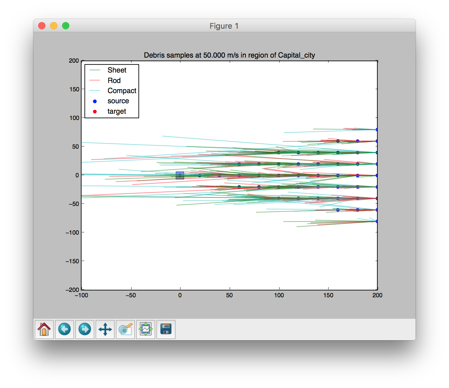
Fig. 15 Test of debris generation function: debris generated at 50 m/s in region of Capcital_city
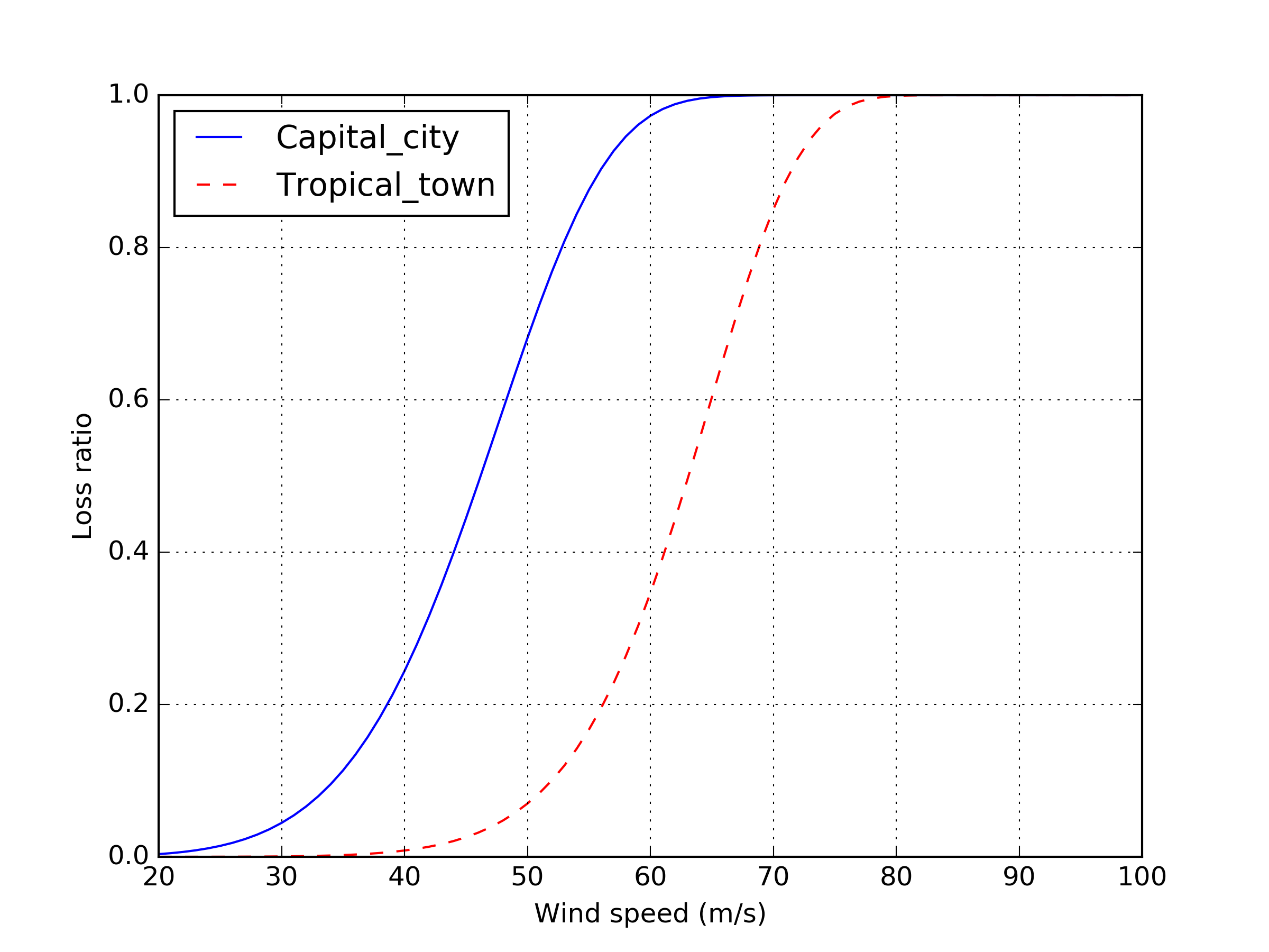
Fig. 16 Vulnerability curves implemented in the debris test function using the parameter values listed in Table 25.
| name | \(\alpha\) | \(\beta\) |
|---|---|---|
| Capital_city | 0.1585 | 3.8909 |
| Tropical_town | 0.1030 | 4.1825 |
The Test button in the Water tab shows relationship between percentage of water ingress and wind speed for a range of damage index as shown in Fig. 17.
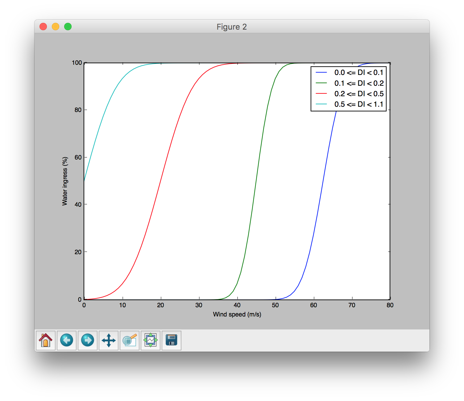
Fig. 17 Relationship between percentage of water ingress and wind speed
Pane #3
This pane contains data browser of house and global data with two tabs at the top: House and Global. The House tab has five tabs at the bottom: Connections, Types, Groups, Zones, and Damage, as shown in Fig. 18. Table 26 sets out corresponding input file and section for each of the tabs.
| Tab name | Input file | Section |
|---|---|---|
| Connections | connections.csv | 3.4.4 connections.csv |
| Types | conn_types.csv | 3.4.3 conn_types.csv |
| Groups | conn_groups.csv | 3.4.2 conn_groups.csv |
| Zones | zones.csv | 3.4.5 zones.csv |
| Damage | damage_costing_data.csv | 3.4.15 damage_costing_data.csv |
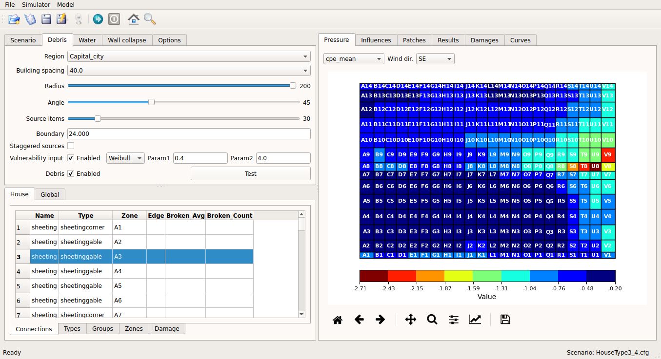
Fig. 18 House data tab showing connections information
The Global tab has two tabs at the bottom: Boundary Profile and Debris, as shown in Fig. 19. In the Boundary Profile tab, gust envelope profiles of selected wind profiles is displayed. Details about the gust envelope profiles can be found in 3.3. In the Debris tab, parameter values for debris model listed in the debris.csv (3.1.3) is displayed. Note that the contents of both tabs are to be changed dynamically upon different selection of wind profile file (Wind Profiles) and debris region (Region).
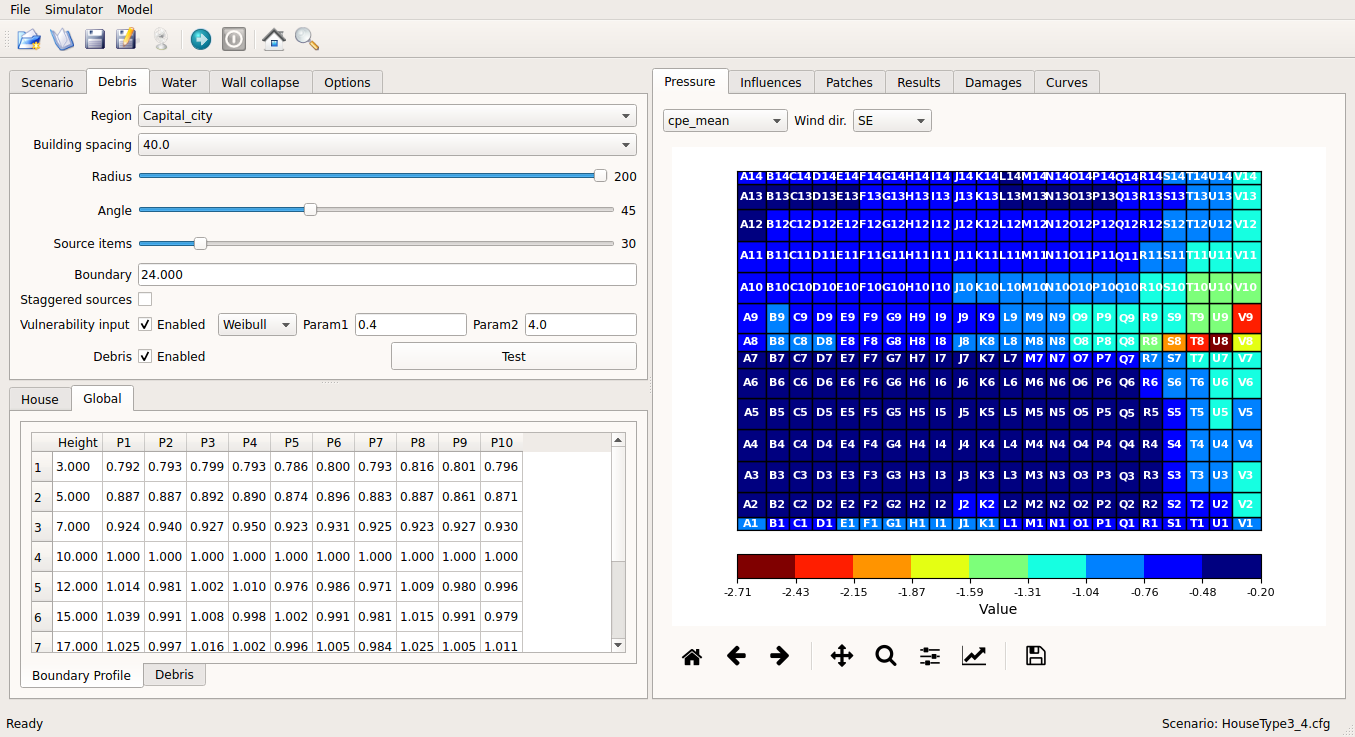
Fig. 19 Global data tab showing boundary profiles information
Pane #4
This pane shows input data of influence coefficients and simulation results. This pane consists of six tabs: Pressure, Influences, Patches, Results, Damages, and Curves, among which Results, Damages, and Curves are empty until a simulation is completed.
Pressure tab
Value of either Cpe_mean (mean \(C_{pe}\)), Cpe_Str_mean (mean \(C_{pe, str}\)), Cpe_eave_mean (mean \(C_{pe, eave}\)), Cpi_alpha (\(C_{pi,\alpha}\)), or Edge of each zone by direction can be shown as Fig. 20.

Fig. 20 Display of value of Cpe_mean for each zone in South-East direction.
Influences tab
Once connection id is set by the slider at the top, then the selected connection (coloured in skyblue) and its associated either zone or connection (coloured in orange) with influence coefficient are shown as Fig. 21.
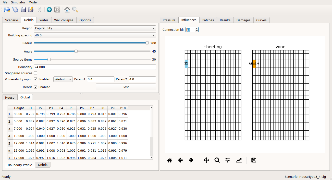
Fig. 21 Display of influence coefficient of connection id 27, which is 1.0 with Zone C3.
Patches tab
The Patches tab shows the influence coefficient of connection when associated connection is failed. Once failed connection (coloured in gray) and connection id (coloured in skyblue) are set, then associated either zone or connection (coloured in orange) with influence coefficient is shown as Fig. 22.
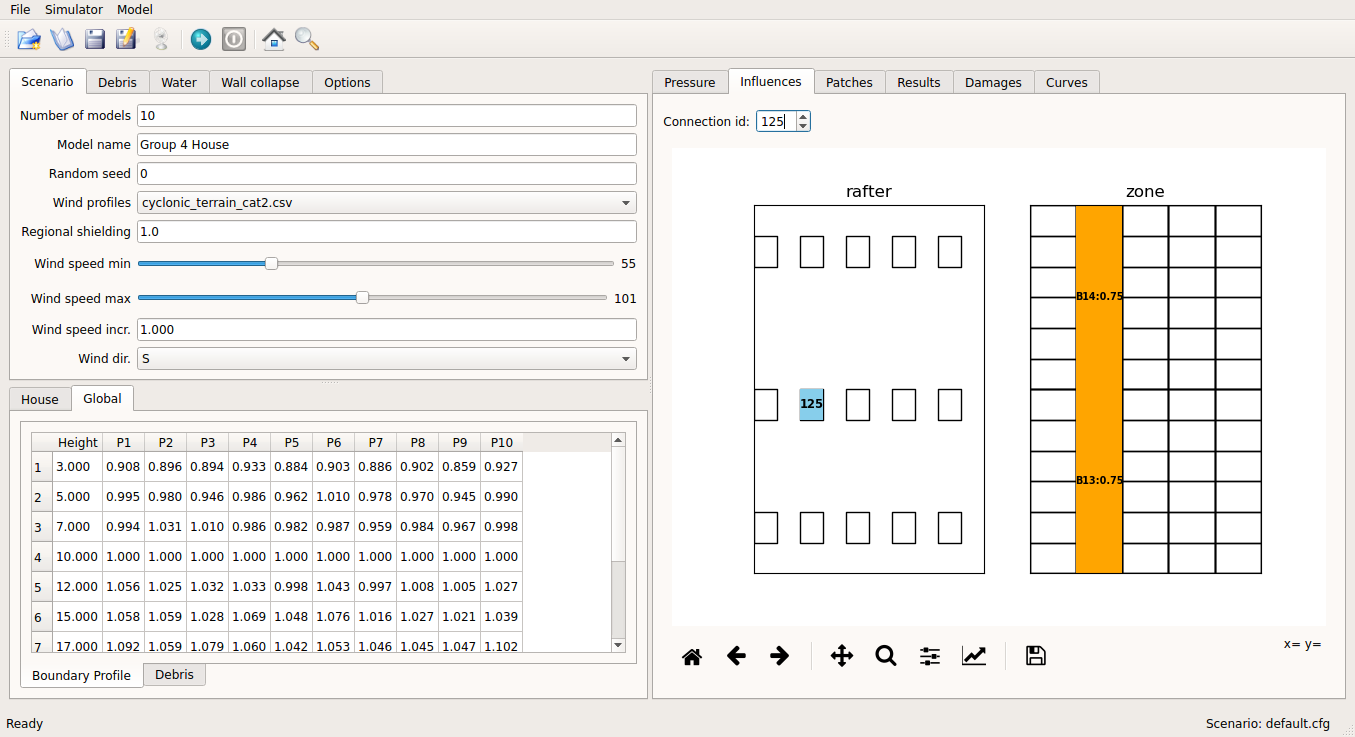
Fig. 22 Display of influence coefficient of connection 125 when connection 124 is failed.
Results tab
The Results tab shows the results of simulation in four sub-windows: Zones, Connections, Type Strengths, Type Damage, and Load.
The Zones window shows sampled Cpe values for each of the zones for each realisation of the simulation models as shown as Fig. 23. The name at the House column consists of model index, and wind direction.
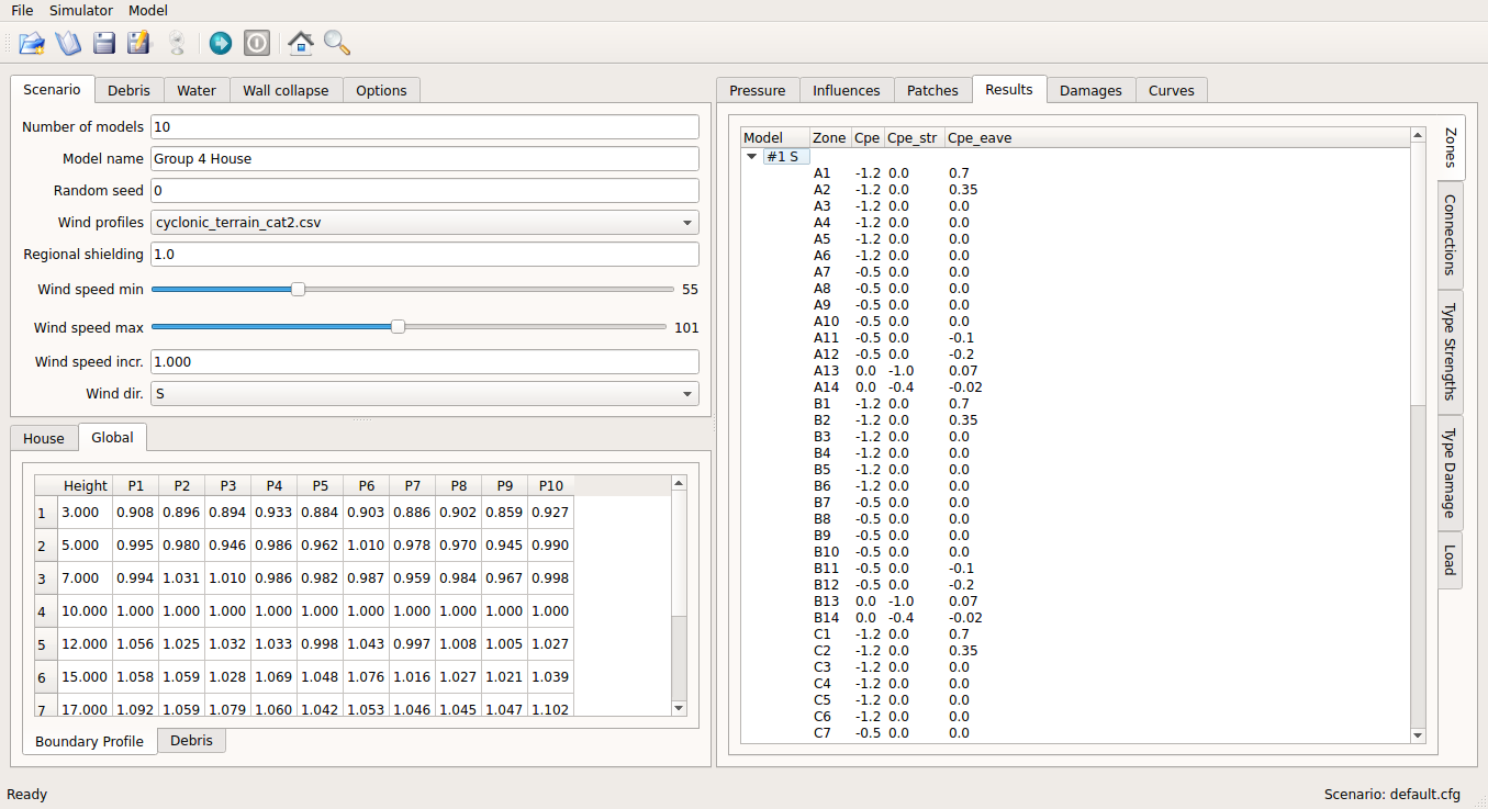
Fig. 23 Display of Cpe values for each zone
Likewise, the Connections window shows the results of each connections such as sampled strength and dead load as shown as Fig. 24.
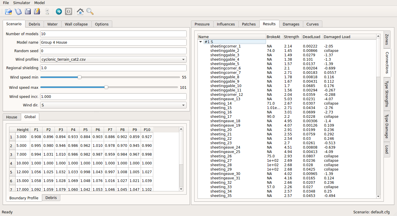
Fig. 24 Display of strength, dead load, and failure wind speed for each connection
The Type Strengths window show distribution of connection strength by connection type as shown as Fig. 25.
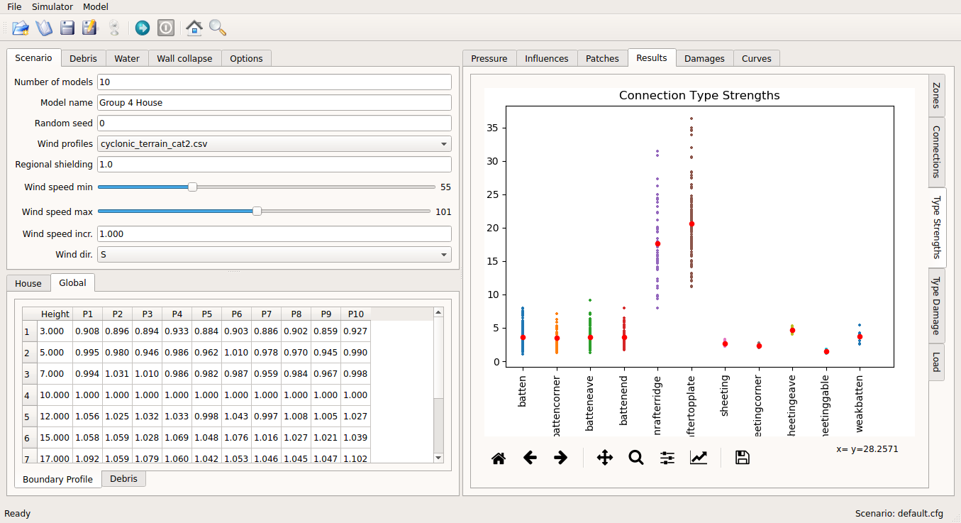
Fig. 25 Display of distribution of sampled connection strength by connection type
The Type Damage window shows distribution of speeds at which connection fails by connection type as shown as Fig. 26.
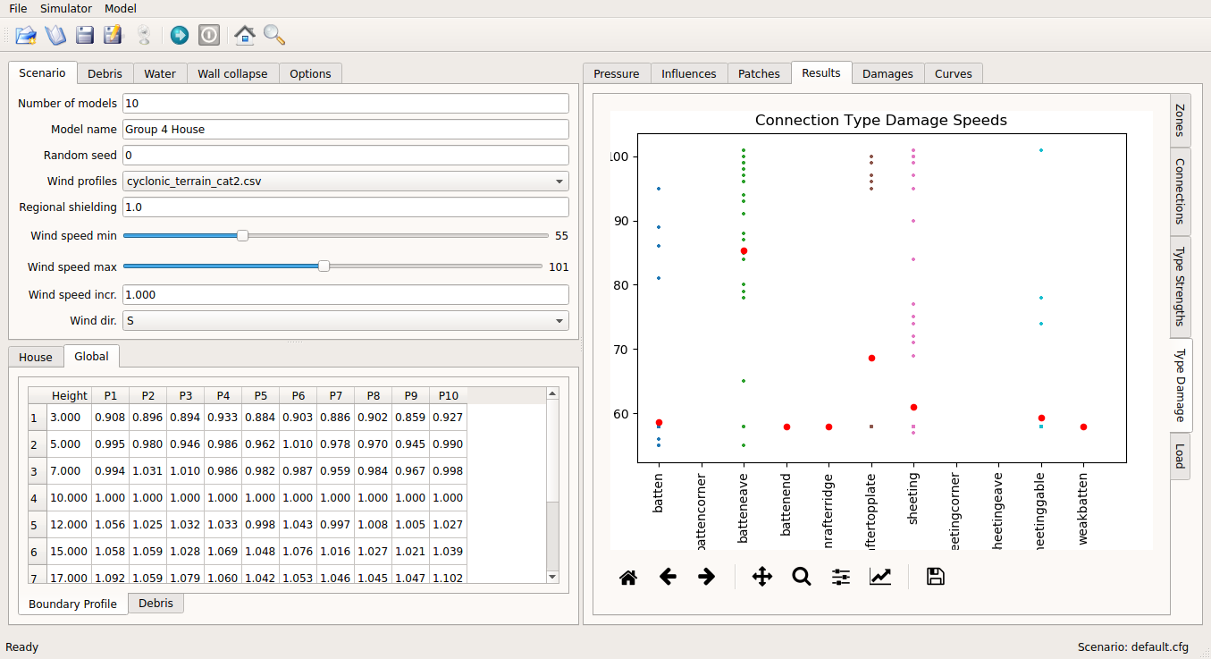
Fig. 26 Display of distribution of failure wind speed by connection type
The Load window shows distribution of speeds at which connection fails by connection type as shown as Fig. 27.

Fig. 27 Display of distribution of ailure wind speed by connection type
Damages tab
The Damages tab shows heatmap by connection type group such as Sheeting, Batten, and Rafter as shown in Fig. 28. The heatmap averaged across models is shown by default, and heatmap for individual model can be displayed by moving the slide at the top.
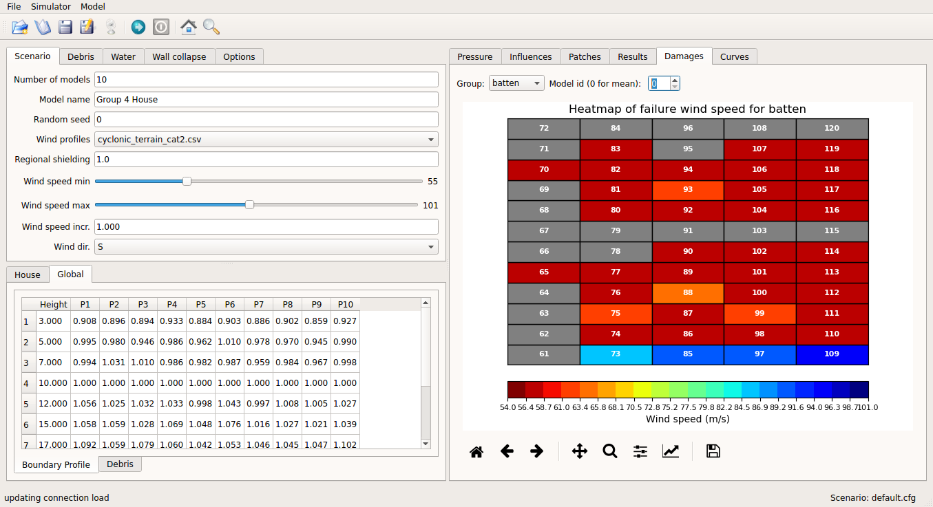
Fig. 28 Heatmap of failure wind speed averaged across models for batten group
Curves tab
The Curves tab shows curves in four sub-windows: Vulnerability, Fragility, Water Ingress, and Debris. The Vulnerability window shows a scatter plot of damage indices at each wind speed along with two fitted vulnerability curves, one of which is cumulative lognormal distribution function as (4) and the other one is cumulative Weibull distribution as (5). The estimated parameter values are displayed at the top.
where \(\Phi\): the cumulative distribution function of the standard normal distribution, \(m\): median, and \(\sigma\): logarithmic standard deviation.
An example plot is shown in Fig. 29.
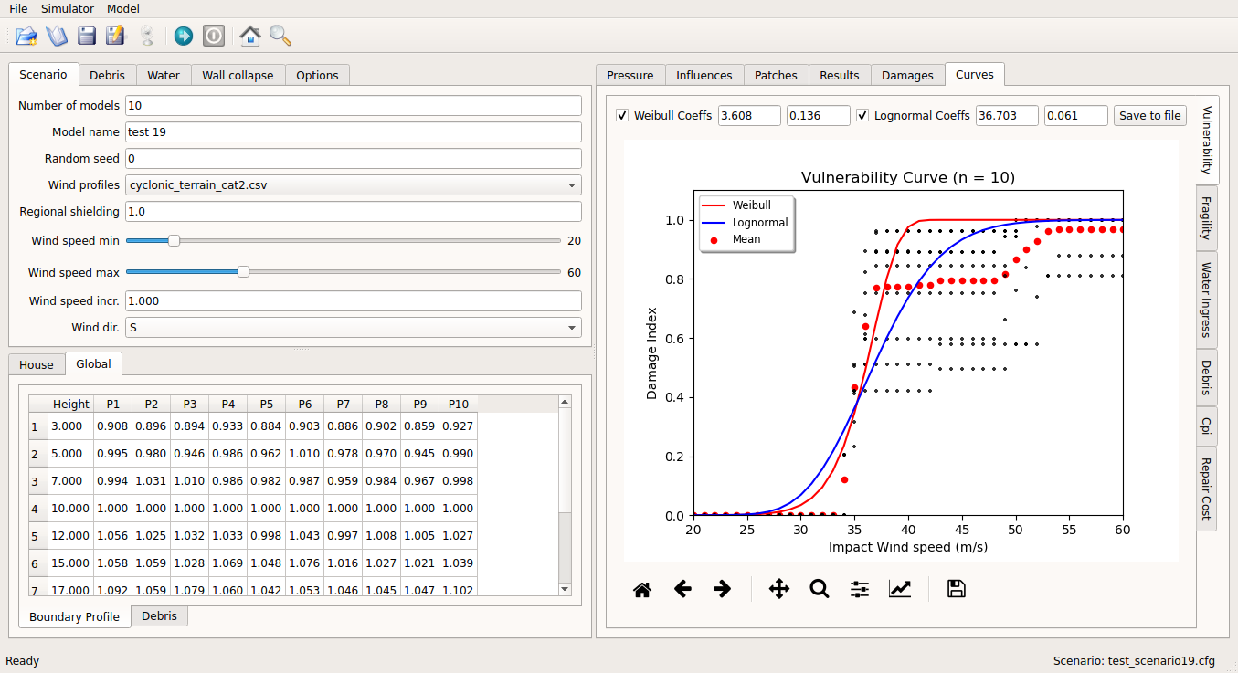
Fig. 29 Plot in the Vulnerability window
The Fragility window shows fragility curves for discrete damage states, which are fitted to cumulative lognormal distribution function, as shown in Fig. 30.
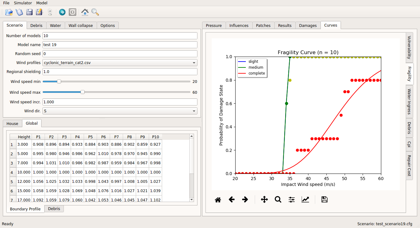
Fig. 30 Plot in the Fragility window
The Water Ingress window shows a scatter plot of the costing associated with water ingress along wind speed, as shown in Fig. 31.
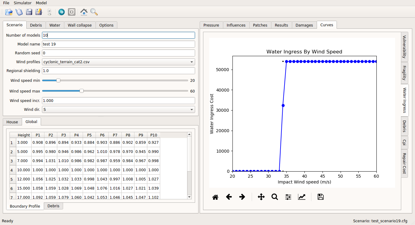
Fig. 31 Plot in the Water Ingress window
The Debris window shows 1) number of generated debris items, 2) number of impacted debris items, and 3) proportion of models breached by debris along the range of wind speed, as shown in Fig. 32.
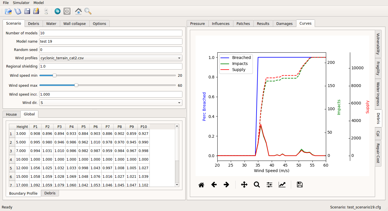
Fig. 32 Plot in the Debris window
The Cpi window shows 1) number of generated debris items, 2) number of impacted debris items, and 3) proportion of models breached by debris along the range of wind speed, as shown in Fig. 33.

Fig. 33 Plot in the Cpi window
The Repair cost window shows 1) number of generated debris items, 2) number of impacted debris items, and 3) proportion of models breached by debris along the range of wind speed, as shown in Fig. 34.

Fig. 34 Plot in the Repair Cost window
Running simulations
The simulation can be run by either 1) creating a new scenario or 2) loading a saved scenario.
Creating a new scenario
User can create a new scenario by clicking the New button, as shown in Table 24. The new scenario comes with a set of input files as an template. Once all the setting are set, then user can save the configuration file to a folder where the template input files will be saved. User need to make changes to each of the input files as required.
Loading a saved scenario
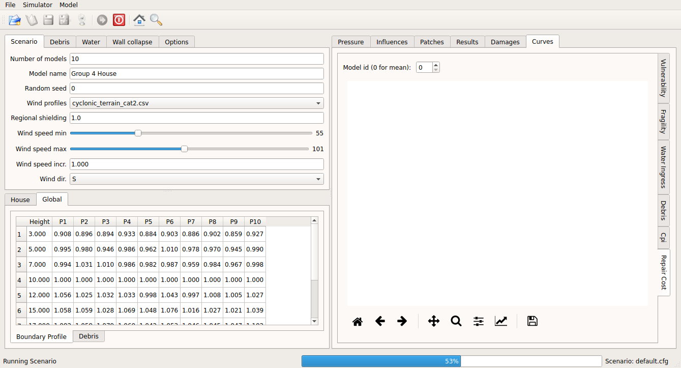
User can load a saved scenario file (e.g., default.cfg). A collection of input files should be located in the directory with the folder structure described in Listing 1. User may make some changes on the settings through GUI. Once all the settings are set, then simulation can be run by clicking the Run button, as shown in Table 24. Once the simulation is completed, user can either exit the program or save the current setting to a different scenario, as shown in Fig. 36.
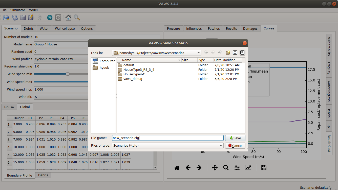
Fig. 36 Save as a new scenario