Input and Output
The input data for a scenario consists of a configuration file and a large number of files located in three different directories. This chapter provides details of input data using the template of default scenario, which can be downloaded from https://github.com/GeoscienceAustralia/vaws/blob/master/scenarios/default. The folder structure of the default scenario is shown Listing 1, which consists of a configuration file (default.cfg) and input directory with three sub-directories (debris, gust_envelope_profiles, and house). The output file named results.h5 is located in the output directory.
 default
 +-- default.cfg
 +-- input
     +-- debris
     |   +-- debris.csv
     |
     +-- gust_envelope_profiles
     |   +-- cyclonic_terrain_cat2.csv
     |   +-- cyclonic_terrain_cat2.5.csv
     |   +-- cyclonic_terrain_cat3.csv
     |   +-- non_cyclonic.csv
     |
     +-- house
         +-- house_data.csv
         +-- conn_groups.csv
         +-- conn_types.csv
         +-- connections.csv
         +-- zones.csv
         +-- zones_cpe_mean.csv
         +-- zones_cpe_str_mean.csv
         +-- zones_cpe_eave_mean.csv
         +-- zones_edge.csv
         +-- coverages.csv
         +-- coverage_types.csv
         +-- coverages_cpe.csv
         +-- influences.csv
         +-- influence_patches.csv
         +-- damage_costing_data.csv
         +-- damage_factorings.csv
         +-- water_ingress_costing_data.csv
         +-- footprint.csv
         +-- front_facing_walls.csv
 +-- output
    +-- results.h5
Configuration file
Each simulation requires a configuration file where basic parameter values for the simulation are provided. The configuration file can be created either by editing the template configuration file using a text editor or through GUI.
The configuration file consists of a number of sections, among which main and options are mandatory while others are optional. An example configuration file is shown in Listing 2.
 [main]
 no_models = 10
 model_name = Group 4 House
 random_seed = 0
 wind_direction = S
 wind_speed_min = 55
 wind_speed_max = 101
 wind_speed_increment = 0.1
 wind_profiles = 'cyclonic_terrain_cat2.csv'
 regional_shielding_factor = 1.0

 [options]
 debris = True
 differential_shielding = False
 water_ingress = True
 debris_vulnerability = True
 wall_collapse = True

 [debris]
 region_name = Capital_city
 staggered_sources = False
 source_items = 250
 boundary_radius = 24.0
 building_spacing = 20.0
 debris_radius = 200
 debris_angle = 45

 [debris_vulnerability]
 function = Weibull
 param1 = 0.4
 param2 = 4.0

 [water_ingress]
 thresholds = 0.1, 0.2, 0.5
 speed_at_zero_wi = 40.0, 35.0, 0.0, -20.0
 speed_at_full_wi = 60.0, 55.0, 40.0, 20.0

 [wall_collapse]
 type_name = rafterwall, collarrafterwall, gablerafterwall
 roof_damage = 0, 25, 50, 75, 100
 wall_damage = 0, 0, 4, 10, 20

 [fragility_thresholds]
 states = slight, medium, severe, complete
 thresholds = 0.02, 0.1, 0.35, 0.9

 [heatmap]
 vmin = 54.0
 vmax = 95.0
 vstep = 21.0
Main section
Parameters of the main section are listed in Table 1. In the GUI window, they are displayed in the Scenario tab as shown in Fig. 2.
| Name | Name in GUI | Description |
|---|---|---|
| no_models | Number of models | number of models |
| model_name | Model name | name of model |
| random_seed | Random seed | a number used to initialize a pseudorandom number generator |
| wind_profiles | Wind profiles | file name of wind profile |
| regional_shielding_factor | Regional shielding | regional shielding factor (default: 1.0) |
| wind_speed_min | Wind speed min | minimum wind speed (m/s) |
| wind_speed_max | Wind speed max | maximum wind speed (m/s) |
| wind_speed_increment | Wind speed incr. | the magnitude of the wind speed increment (m/s) |
| wind_direction | Wind dir. | wind direction (S, SW, W, NW, N, NE, E, SE, or RANDOM) |
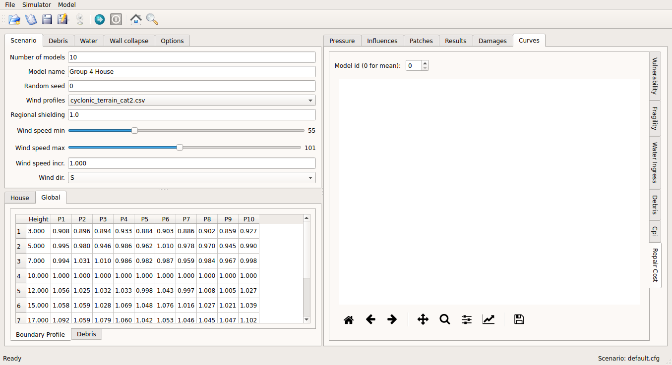
Fig. 2 Parameters of main section in the Scenario tab
Options section
Parameters of the Options section are listed in Table 2. Note that all the parameter values of the option section should be chosen between True (or 1) or False (or 0). In the GUI window, they are displayed in the Debris, Water, and Options tab as listed in the Table 2.
| Name | Name in GUI | Description |
|---|---|---|
| debris | ‘Enabled’ tick box in the Debris tab | if True then debris damage will be simulated. |
| differential_shielding | ‘Differential shielding’ tick box in the Options tab | if True then differential shielding effect is applied. |
| debris_vulnerability | ‘Enabled’ tick box in the Debris tab | if True then input vulnerability will be used in debris generation. |
| water_ingress | ‘Enabled’ tick box in the Water tab | if True then damage due to water ingress will be simulated. |
| wall_collapse | ‘Enabled’ tick box in the Wall collapse tab | if True then wall collapse will be simulated. |
| save_heatmaps | ‘Save heatmaps’ tick box in the Options tab | if True then heatmap plot of each model will be saved. |
Debris section
Parameters of the debris section are listed in Table 3. Note that debris section is only required if debris is set to be True in the options. In the GUI window, they are displayed in the Debris tab as shown in Fig. 3.
| Name | Name in GUI | Description |
|---|---|---|
| region_name | Region | one of the region names defined in the Listing 3. Each region has different debris source characteristics. |
| building_spacing | Building spacing | distance between debris sources (m) |
| debris_radius | Radius | radius (in metre) of debris sources from the modelled house |
| debris_angle | Angle | included angle (in degree) of the sector in which debris sources exist |
| source_items | Source items | number of debris items per debris sources |
| boundary_radius | Boundary | radius (in metre) of boundary for debris impact assessment |
| staggered_sources | Staggered sources | if True then staggered sources are used. Otherwise, a grid pattern of debris sources are used. |
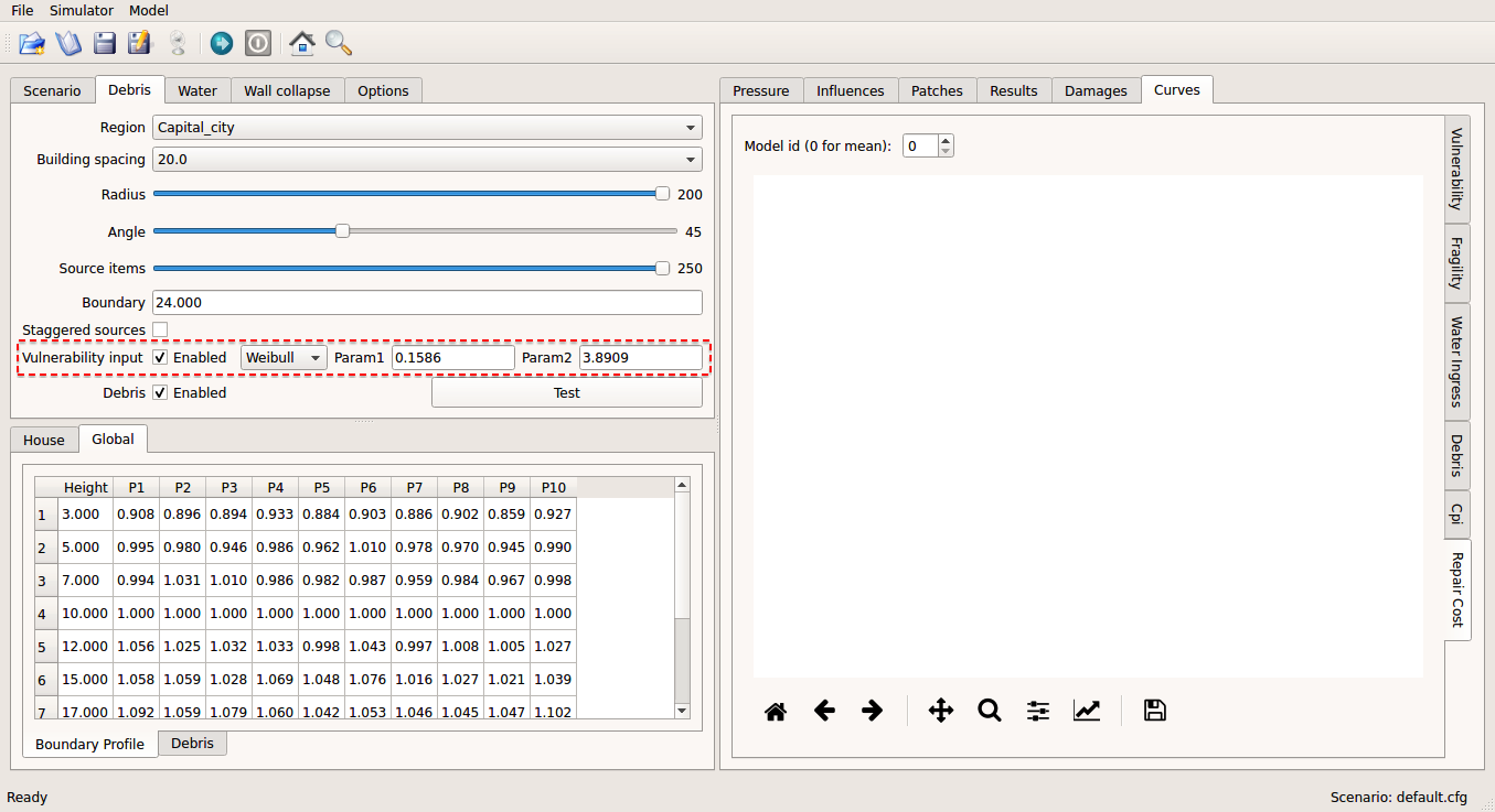
Fig. 3 Parameters of debris section in Debris tab
Debris vulnerability section
Parameters of the debris vulnerability section are listed in Table 4. Note that debris vulnerability section is only required if debris_vulnerability is set to be True in the options. In the GUI window, they are displayed in the Debris tab as box shown in Fig. 3.
| Name | Name in GUI | Description |
|---|---|---|
| function | Vulnerability input | Weibull (5) or Lognorm (4) distribution. |
| param1 | Param1 | \(\alpha\) for Weibull or \(m\) for Lognormal distribution |
| param2 | Param2 | \(\beta\) for Weibull or \(\sigma\) for Lognormal distribution |
Water_ingress section
Parameters of the water_ingress section are listed in Table 5. In the GUI window, they are displayed in the Water tab as shown in Fig. 5. The thresholds define a lower limit of envelope damage index above which the relevant water ingress vs wind speed curve is applied. The speeds at 0% water ingress and speeds at 100% water ingress define cumulative normal distribution used to relate percentage water ingress to wind speed as shown in Fig. 4.
| Name | Name in GUI | Description |
|---|---|---|
| thresholds | DI thresholds | comma separated list of thresholds of damage indices (default: 0.1, 0.2, 0.5) |
| speed_at_zero_wi | Speeds at 0% WI | comma separated list of maximum wind speed at no water ingress (default: 40.0, 35.0, 0.0, -20.0) |
| speed_at_full_wi | Speeds at 100% WI | comma separated list of minimum wind speed at full water ingress (default: 60.0, 55.0, 40.0, 20.0) |
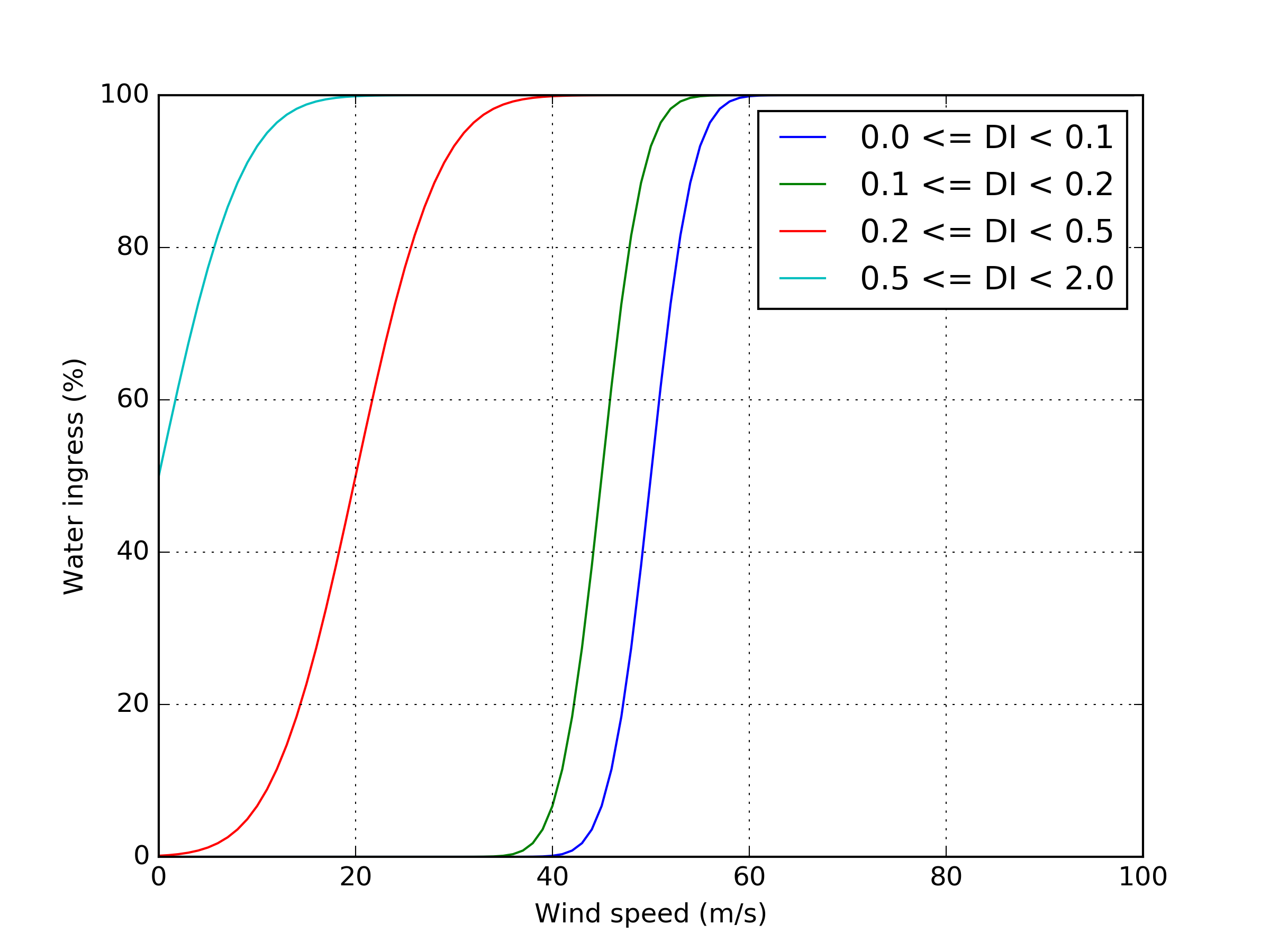
Fig. 4 Water ingress vs. wind speed for different ranges of damage index
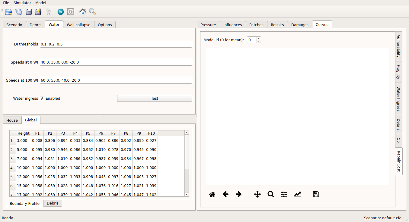
Fig. 5 Parameters of water_ingress section in Water tab
Wall collapse section
Parameters of the wall_collapse section are listed in Table 6. In the GUI window, they are displayed in the Wall collapse tab as shown in Fig. 6.
| Name | Name in GUI | Description |
|---|---|---|
| type_name | Type name | comma separated list of name of connection types |
| roof_damage | Roof damage (%) | comma separated list of percentage of roof damage |
| wall_damage | Wall damage(%) | comma separated list of percentage of wall damage |

Fig. 6 Parameters of wall collapse section in wall collapse tab

Fig. 7 Prediction of wall damage given roof damage
Fragility_thresholds
Parameters of the fragility_thresholds section are listed in Table 7. In the GUI window, they are displayed in the Options tab as shown in Fig. 8. The fragility thresholds are used as shown in (25).
| Name | Name in GUI | Description |
|---|---|---|
| states | Damage states | comma separated list of damage states (default: slight, medium, severe, complete) |
| thresholds | Thresholds | comma separated list of damage states thresholds (default: 0.02, 0.1, 0.35, 0.9) |
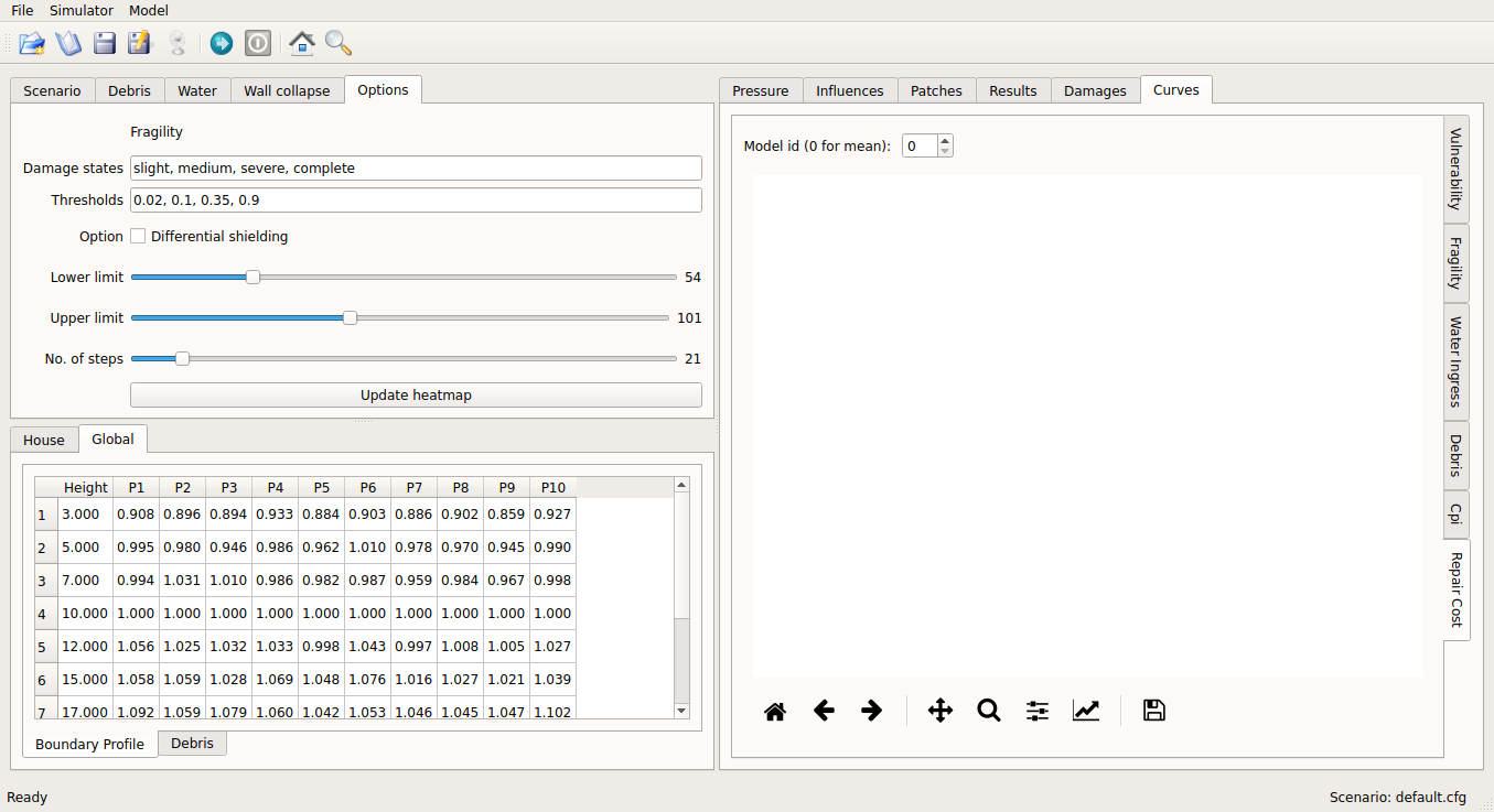
Fig. 8 Parameters of fragility_thresholds section in Options tab
Heatmap
Parameters of the heatmap section are listed in Table 8. In the GUI window, they are displayed in the Options tab as shown in Fig. 9
| Name | Name in GUI | Description |
|---|---|---|
| vmin | Lower limit | lower limit of wind speed for heatmap |
| vmax | Upper limit | upper limit of wind speed for heatmap |
| vstep | No. of steps | number of steps |

Fig. 9 Parameters of heatmap section in Options tab
Input file under debris directory
In the debris directory, debris.csv is located where parameter values related to windborne debris are defined. Three types of windborne debris are modelled, as listed in Table 9, which include Compact, Rod, and Sheet. Parameter values for each debris type needs to be defined by unique region name, and the defined region name should be referenced in the configuration file.
An example debris.csv is shown in Listing 3, in which debris parameters are defined for both Capital_city and Tropical_town. Note that Capital_city is referenced in the example configuration file Listing 2.
 Region name,Capital_city,Tropical_town
 Compact_ratio,20,15
 Compact_mass_mean,0.1,0.1
 Compact_mass_stddev,0.1,0.1
 Compact_frontal_area_mean,0.002,0.002
 Compact_frontal_area_stddev,0.001,0.001
 Compact_cdav,0.65,0.65
 Compact_flight_time_mean, 2.0, 2.0
 Compact_flight_time_stddev, 0.8, 0.8
 Rod_ratio,30,40
 Rod_mass_mean,4,4
 Rod_mass_stddev,2,2
 Rod_frontal_area_mean,0.1,0.1
 Rod_frontal_area_stddev,0.03,0.03
 Rod_cdav,0.8,0.8
 Rod_flight_time_mean, 2.0, 2.0
 Rod_flight_time_stddev, 0.8, 0.8
 Sheet_ratio,50,45
 Sheet_mass_mean,3,10
 Sheet_mass_stddev,0.9,5
 Sheet_frontal_area_mean,0.1,1
 Sheet_frontal_area_stddev,0.03,0.3
 Sheet_cdav,0.9,0.9
 Sheet_flight_time_mean, 2.0, 2.0
 Sheet_flight_time_stddev, 0.8, 0.8
| Name | Examples |
|---|---|
| Compact | Loose nails screws, washers, parts of broken tiles, chimney bricks, air conditioner units |
| Rod | Parts of timber battens, purlins, rafters |
| Sheet | Roof cladding (mainly tiles, steel sheet, flashing, solar panels) |
The parameter values should be provided for each of the debris types as set out in Table 10.
| Name | Note |
|---|---|
| ratio | proportion out of debris in percent |
| mass_mean | mean of mass (kg) |
| mass_stddev | standard deviation of mass (kg) |
| frontal_area_mean | mean of frontal area (\(\text{m}^2\)) |
| frontal_area_stddev | standard deviation of frontal area (\(\text{m}^2\)) |
| cdav | average drag coefficient |
| flight_time_mean | mean of flight time (sec) |
| frontal_area_stddev | standard deviation of flight time (sec) |
Input files under gust_envelope_profiles directory
The gust envelope profiles are defined under gust_envelope_profiles directory. In the configuration file, file name of the gust envelope profile needs to be referenced as shown in Listing 2.
Example files are provided with respect to Australian wind design categories: cyclonic_terrain_cat2.csv, cyclonic_terrain_cat2.5.csv, cyclonic_terrain_cat3.csv, and non_cyclonic.csv, which are recommended in JDH Consulting, 2010 [3].
An example of gust envelope profile is provided in Listing 4, and the corresponding plot is shown in Fig. 10.
 # Terrain Category 2
 3,0.908,0.896,0.894,0.933,0.884,0.903,0.886,0.902,0.859,0.927
 5,0.995,0.980,0.946,0.986,0.962,1.010,0.978,0.970,0.945,0.990
 7,0.994,1.031,1.010,0.986,0.982,0.987,0.959,0.984,0.967,0.998
 10,1.000,1.000,1.000,1.000,1.000,1.000,1.000,1.000,1.000,1.000
 12,1.056,1.025,1.032,1.033,0.998,1.043,0.997,1.008,1.005,1.027
 15,1.058,1.059,1.028,1.069,1.048,1.076,1.016,1.027,1.021,1.039
 17,1.092,1.059,1.079,1.060,1.042,1.053,1.046,1.045,1.047,1.102
 20,1.110,1.103,1.037,1.068,1.088,1.107,1.068,1.106,1.098,1.103
 25,1.145,1.151,1.069,1.091,1.089,1.196,1.126,1.113,1.099,1.142
 30,1.245,1.188,1.177,1.178,1.192,1.199,1.179,1.165,1.127,1.203
The first row is header, and heights (in metre) are listed in the first column. Profile values along the heights are listed from the second column with comma separation. One wind profile (one column) will be randomly selected for each run of the simulation.
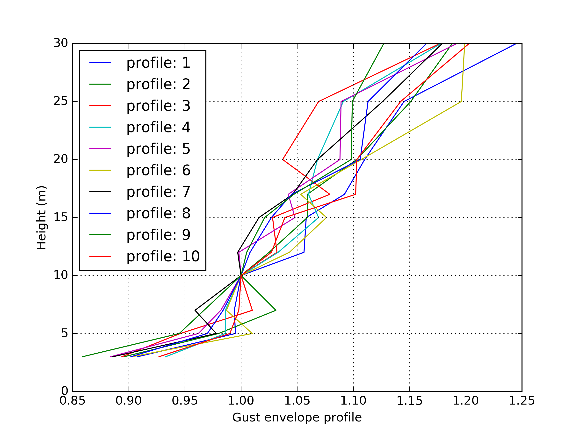
Fig. 10 Wind gust envelope profile along height.
Input files under house directory
In the house directory, a large number of files are located which are required to set parameter values of the model. The simulation model is assumed to consist of connections, zones, and coverages. The connections are grouped into a number of connection types, and the connection types are further grouped into connection groups.
house_data.csv
This file defines parameter values for the model such as replacement cost and dimensions. An example is shown in Listing 5, and description of each of the parameter values are provided in Table 11.
 replace_cost,3220.93
 height,4.5
 length,0.9
 width,9.0
 cpe_cv,0.0
 cpe_k,0.1
 cpe_str_cv,0.0
 cpe_str_k,0.1
| Name | Type | Description |
|---|---|---|
| replace_cost | float | replacement cost of the model ($) |
| height | float | height of the model (in metre) |
| length | float | length of the model (in metre) |
| width | float | width of the model (in metre) |
| cpe_cv | float | CV of \(C_{pe}\) for cladding elements such as sheeting and batten |
| cpe_k | float | shape factor of \(C_{pe}\) for cladding elements such as sheeting and batten |
| cpe_str_cv | float | CV of \(C_{pe,str}\) for structural elements such as rafter |
| cpe_str_k | float | shape factor of \(C_{pe,str}\) for structural elements as rafter |
conn_groups.csv
The model is assumed to consist of a number of connection groups. This file defines connection groups and parameter values of the each connection group. An example is shown in Listing 6, and description of each of the parameter values are provided in Table 12.
 group_name,dist_order,dist_dir,damage_dist,damage_scenario,trigger_collapse_at,flag_pressure
 sheeting,1,col,1,Loss of roof sheeting,0.0,cpe
 batten,2,row,1,Loss of roof sheeting & purlins,0.0,cpe
 rafter,3,patch,1,Loss of roof structure,0.0,cpe_str
| Name | Type | Description |
|---|---|---|
| group_name | string | name of connections group |
| dist_order | integer | order of checking damage |
| dist_dir | string | direction of damage distribution; either ‘col’, ‘row’, ‘patch’, or ‘none |
| damage_dist | integer | 1 if load distribution is applied when connection is damaged otherwise 0 |
| damage_scenario | string | damage scenario name defined in damage_costing_data.csv |
| trigger_collapse_at | float | proportion of damaged connections of the group at which a model is deemed to be collapsed. 0 if ignored |
| flag_pressure | string | type of \(C_{pe}\) for pressure calculation; either ‘cpe’ or ‘cpe_str’ |
conn_types.csv
A connection group may consists of a number of connection types which have different parameter values for strength, dead load, and costing area. This file defines connection types and parameter values of the each connection type. An example is shown in Listing 7, and description of each of the parameter values are provided in Table 13.
 type_name,strength_mean,strength_std,dead_load_mean,dead_load_std,group_name,costing_area
 sheetinggable,1.54,0.16334,0.02025,0.0246,sheeting,0.405
 sheetingeave,4.62,0.28292,0.02025,0.0246,sheeting,0.405
 sheetingcorner,2.31,0.2,0.01013,0.0246,sheeting,0.225
 sheeting,2.695,0.21608,0.0405,0.0246,sheeting,0.81
 batten,3.6,1.26,0.089,0.0708,batten,0.81
 battenend,3.6,1.26,0.089,0.0708,batten,0.405
 batteneave,3.6,1.26,0.089,0.0708,batten,0.405
 battencorner,3.6,1.26,0.089,0.0708,batten,0.225
 endraftertopplate,19.5,5.85,0.84,0.063,rafter,1.238
 endrafterridge,16.5,4.95,1.8,0.135,rafter,1.665
 collarraftertopplate,19.5,5.85,1.68,0.126,rafter,1.845
 collarrafterridge,16.5,4.95,1.13,0.08475,rafter,1.26
 collarraftercollar,2.4,0.48,3.95,0.29625,rafter,1.665
 plainraftertopplate,19.5,5.85,1.68,0.126,rafter,2.475
 plainrafterridge,16.5,4.95,3.6,0.27,rafter,3.33
 weakbatten,3.6,1.26,0.089,0.0708,batten,0.81
| Name | Type | Description |
|---|---|---|
| type_name | string | name of connection type |
| strength_mean | float | mean strength (kN) |
| strength_std | float | standard deviation of strength |
| dead_load_mean | float | mean dead load (kN) |
| dead_load_std | float | standard deviation of dead load |
| group_name | string | name of connections group |
| costing_area | float | costing area (\(\text{m}^2\)) |
connections.csv
This file defines connections and parameter values of the each connection. An example is shown in Listing 8, and description of each of the parameter values are provided in Table 14.
 conn_name,type_name,zone_loc,section,coords
 1,sheetingcorner,A1,1,0,0,0.2,0,0.2,0.5,0,0.5
 2,sheetinggable,A2,1,0,0.5,0.2,0.5,0.2,1,0,1
 3,sheetinggable,A3,1,0,1,0.2,1,0.2,1.5,0,1.5
 4,sheetinggable,A4,1,0,1.5,0.2,1.5,0.2,2,0,2
 5,sheetinggable,A5,1,0,2,0.2,2,0.2,2.5,0,2.5
| Name | Type | Description |
|---|---|---|
| conn_name | string | name of connection |
| type_name | string | name of connection type |
| zone_loc | integer | zone name corresponding to connection location |
| section | integer | index of section in which damage distribution occurs |
| coords | float | comma separated values of x, y coordinates for plotting purpose. e.g., 4 sets for a rectangular shape, 3 sets for a triangular shape. |
zones.csv
This file defines zones and parameter values of the each zone. An example is shown in Listing 9, and description of each of the parameter values are provided in Table 15.
 name,area,cpi_alpha,coords,
 A1,0.2025,0,0,0,0.2,0,0.2,0.5,0,0.5
 A2,0.405,0.5,0,0.5,0.2,0.5,0.2,1,0,1
 A3,0.405,1,0,1,0.2,1,0.2,1.5,0,1.5
 A4,0.405,1,0,1.5,0.2,1.5,0.2,2,0,2
 A5,0.405,1,0,2,0.2,2,0.2,2.5,0,2.5
| Name | Type | Description |
|---|---|---|
| name | string | name of zone |
| area | float | area of zone (\(\text{m}^2\)) |
| cpi_alpha | float | proportion of the zone’s area to which internal pressure is applied |
| coords | float | comma separated list of x, y coordinates for plotting purpose. e.g., 4 sets for a rectangular shape, 3 sets for a triangular shape. |
zones_cpe_mean.csv
This file defines mean cladding \(C_{pe}\) of each zone with regard to the eight wind directions. An example is shown in Listing 10, and description of each of the parameter values are provided in Table 16.
 name,S,SW,W,NW,N,NE,E,SE
 A1,-1.2,-1.2,-1.2,-1.2,-1.2,-1.2,-1.2,-1.2
 A2,-1.2,-1.2,-1.2,-1.2,-1.2,-1.2,-1.2,-1.2
 A3,-1.2,-1.2,-1.2,-1.2,-1.2,-1.2,-1.2,-1.2
 A4,-1.2,-1.2,-1.2,-1.2,-1.2,-1.2,-1.2,-1.2
 A5,-1.2,-1.2,-1.2,-1.2,-1.2,-1.2,-1.2,-1.2
 A6,-1.2,-1.2,-1.2,-1.2,-1.2,-1.2,-1.2,-1.2
 A7,-0.5,-0.5,-0.5,-0.5,-0.5,-0.5,-0.5,-0.5
 A8,-0.5,-0.5,-0.5,-0.5,-0.5,-0.5,-0.5,-0.5
 A9,-0.5,-0.5,-0.5,-0.5,-0.5,-0.5,-0.5,-0.5
 A10,-0.5,-0.5,-0.5,-0.5,-0.5,-0.5,-0.5,-0.5
 A11,-0.5,-0.5,-0.5,-0.5,-0.5,-0.5,-0.5,-0.5
 A12,-0.5,-0.5,-0.5,-0.5,-0.5,-0.5,-0.5,-0.5
 A13,0,0,0,0,0,0,0,0
 A14,0,0,0,0,0,0,0,0
| Name | Type | Description |
|---|---|---|
| name | string | name of zones |
| S | float | mean cladding \(C_{pe}\) value in South direction |
| SW | float | mean cladding \(C_{pe}\) value in South West direction |
| W | integer | mean cladding \(C_{pe}\) value in West direction |
| NW | float | mean cladding \(C_{pe}\) value in North East direction |
| N | float | mean cladding \(C_{pe}\) value in North direction |
| NE | float | mean cladding \(C_{pe}\) value in North East direction |
| E | integer | mean cladding \(C_{pe}\) value in East direction |
| SE | float | mean cladding \(C_{pe}\) value in South East direction |
zones_cpe_str_mean.csv
Like zones_cpe_mean.csv, mean \(C_{pe,str}\) values for zones associated with structural component (e.g., rafter) need to be provided in zones_cpe_str_mean.csv. An example is shown in Listing 11.
 name,S,SW,W,NW,N,NE,E,SE
 A1,0,0,0,0,0,0,0,0
 A2,0,0,0,0,0,0,0,0
 A3,0,0,0,0,0,0,0,0
 A4,0,0,0,0,0,0,0,0
 A5,0,0,0,0,0,0,0,0
 A6,0,0,0,0,0,0,0,0
 A7,0,0,0,0,0,0,0,0
 A8,0,0,0,0,0,0,0,0
 A9,0,0,0,0,0,0,0,0
 A10,0,0,0,0,0,0,0,0
 A11,0,0,0,0,0,0,0,0
 A12,0,0,0,0,0,0,0,0
 A13,-1,-1,-1,-1,-1,-1,-1,-1
 A14,-0.4,-0.4,-0.4,-0.4,-0.4,-0.4,-0.4,-0.4
zones_cpe_eave_mean.csv
Like zones_cpe_mean.csv, mean \(C_{pe}\) values for zones at eave need to be provided in zones_cpe_eave_mean.csv. An example is shown in Listing 12.
 name,S,SW,W,NW,N,NE,E,SE
 A1,0.7,0.7,0.7,0.7,0.7,0.7,0.7,0.7
 A2,0.35,0.35,0.35,0.35,0.35,0.35,0.35,0.35
 A3,0,0,0,0,0,0,0,0
 A4,0,0,0,0,0,0,0,0
 A5,0,0,0,0,0,0,0,0
 A6,0,0,0,0,0,0,0,0
 A7,0,0,0,0,0,0,0,0
 A8,0,0,0,0,0,0,0,0
 A9,0,0,0,0,0,0,0,0
 A10,0,0,0,0,0,0,0,0
 A11,-0.1,-0.1,-0.1,-0.1,-0.1,-0.1,-0.1,-0.1
 A12,-0.2,-0.2,-0.2,-0.2,-0.2,-0.2,-0.2,-0.2
 A13,0.07,0.07,0.07,0.07,0.07,0.07,0.07,0.07
 A14,-0.02,-0.02,-0.02,-0.02,-0.02,-0.02,-0.02,-0.02
zones_edge.csv
In zones_edge.csv, for each of the eight direction, 1 is provided for zone within the region of a roof edge, otherwise 0. Zones in the edge region are considered to be subjected to differential shielding if enabled by user. An example is shown in Listing 13.
 name,S,SW,W,NW,N,NE,E,SE
 A1,1,1,1,0,0,0,0,0
 A2,1,1,1,0,0,0,0,0
 A3,1,1,1,0,0,0,0,0
 A4,0,1,0,0,0,0,0,0
 A5,0,1,0,0,0,0,0,0
 A6,0,1,0,0,0,0,0,0
 A7,0,0,0,1,0,0,0,0
 A8,0,0,0,1,0,0,0,0
 A9,0,0,0,1,0,0,0,0
 A10,0,0,1,1,1,0,0,0
 A11,0,0,1,1,1,0,0,0
 A12,0,0,1,1,1,0,0,0
 A13,1,1,1,0,0,0,0,0
 A14,0,0,1,1,1,0,0,0
coverages.csv
This file defines coverages making up the wall part of the envelope of the model. An example is shown in Listing 14, and description of each of the parameter values are provided in Table 17. The wall name is defined in Listing 23. Coverages are assessed for debris impact damage and failure by direct wind pressure. The area of coverage is used in the calculation of \(C_{pi}\).
 name,description,wall_name,area,coverage_type,repair_type
 1,window,1,3.6,Glass_annealed_6mm,full
 2,door,1,1.8,Timber_door,full
 3,window,1,1.89,Glass_annealed_6mm,full
 4,window,1,1.89,Glass_annealed_6mm,full
 5,weatherboard,1,22.02,Weatherboard,partial
| Name | Type | Description |
|---|---|---|
| name | integer | coverage index |
| description | string | description |
| wall_name | integer | wall name |
| area | float | area (\(\text{m}^2\)) |
| coverage_type | string | name of coverage type |
| repiar_type | string | full or partial depending on the extent of repiar |
coverage_types.csv
This file defines types of coverages referenced in the Listing 14. An example is shown in Listing 15, and description of each of the parameter values are provided in Table 18.
 name,failure_momentum_mean,failure_momentum_std,failure_strength_in_mean,failure_strength_in_std,failure_strength_out_mean,failure_strength_out_std
 Glass_annealed_6mm,0.05,0.0,100,0.0,-100,0.0
 Timber_door,142.2,28.44,100,0.0,-100,0.0
| Name | Type | Description |
|---|---|---|
| name | string | name of coverage type |
| failure_momentum_mean | float | mean failure momentum (\(\text{kg}\cdot\text{m/s}\)) for debris impact |
| failure_momentum_std | float | standard deviation of failure momentum |
| failure_strength_in_mean | float | mean failure strength inward direction (positive) for failure due to wind pressure (kN) |
| failure_strength_in_std | float | standard deviation of failure strength inward direction |
| failure_strength_out_mean | float | mean failure strength outward direction (negative) for failure due to wind pressure (kN) |
| failure_strength_out_std | float | standard deviation of failure strength outward direction |
coverages_cpe.csv
Like zones_cpe_mean.csv, mean \(C_{pe}\) values for coverages are provided in coverages_cpe.csv. An example is shown in Listing 16.
 ID,S,SW,W,NW,N,NE,E,SE
 1,2.4,2.4,2.4,2.4,2.4,2.4,2.4,2.4
 2,1.69,1.69,1.69,1.69,1.69,1.69,1.69,1.69
 3,-1.14,-1.14,-1.14,-1.14,-1.14,-1.14,-1.14,-1.14
 4,-1.45,-1.45,-1.45,-1.45,-1.45,-1.45,-1.45,-1.45
 5,0.9,0.9,0.9,0.9,0.9,0.9,0.9,0.9
 6,-0.55,-0.55,-0.55,-0.55,-0.55,-0.55,-0.55,-0.55
influences.csv
This file defines influence coefficients relating a connection with either another connection(s) or zone(s). The wind load acting on a connection can be computed as the sum of the product of influence coefficient and either wind load on zone or load on another connection. An example is shown in Listing 17, and description of each of the parameter values are provided in Table 19. In this example, connection 1 is related to the zone A1 with coefficient 1.0, and connection 61 is related to the connection 1 with coefficient 1.0. Similarly, connection 121 is related to the zone A13 with coefficient 0.81 and the zone A14 with coefficient 0.19.
 Connection,Zone,Coefficent
 1,A1,1.0
 2,A2,1.0
 61,1,1
 62,2,1
 63,3,1
 121,A13,0.81,A14,0.19
| Name | Description |
|---|---|
| Connection | name of connection |
| Zone | name of either zone or connection associated with the Connection |
| Coefficient | coefficient value |
influence_patches.csv
This file defines influence coefficients of connections when associated connection is failed. An example is shown in Listing 18, and description of each of the parameter values are provided in Table 20. In the example, when connection 121 is failed, influence coefficients of connection 121, 122, 123 are re-defined.
 Damaged connection,Connection,Zone,Coefficient
 121,121,A13,0,A14,0
 121,122,A13,1,A14,0
 121,123,A13,1,A14,1
 122,121,A13,1,A14,0
 122,122,A13,0,A14,0
 122,123,A13,0,A14,1
| Name | Description |
|---|---|
| Damaged Connection | name of damaged connection |
| Connection | name of connection for which the influence coefficients are to be updated |
| Zone | name of either zone or connection associated with the connection to be updated |
| Coefficient | new influence coefficient value |
damage_costing_data.csv
This file defines damage scenarios referenced in Listing 6. An example is shown in Listing 19, and description of each of the parameter values are provided in Table 21. The damage cost for each damage scenario \(C\) is calculated as
where \(x\): proportion of damaged area (\(0 \leq x \leq 1\)), \(A\): surface area, \(C_\text{env}\): costing function for envelope, \(R_\text{env}\): repair rate for envelope, \(C_\text{int}\): costing function for internal, and \(R_\text{int}\): repair rate for internal. Two types of costing functions are defined as:
 name,surface_area,envelope_repair_rate,envelope_factor_formula_type,envelope_coeff1,envelope_coeff2,envelope_coeff3,internal_repair_rate,internal_factor_formula_type,internal_coeff1,internal_coeff2,internal_coeff3,water_ingress_order
 Loss of roof sheeting,116,72.4,1,0.3105,-0.8943,1.6015,0,1,0,0,0,6
 Loss of roof sheeting & purlins,116,184.23,1,0.3105,-0.8943,1.6015,0,1,0,0,0,7
 Loss of roof structure,116,317,1,0.3105,-0.8943,1.6015,8320.97,1,-0.4902,1.4896,0.0036,3
| Name | Description |
|---|---|
| name | name of damage scenario |
| surface_area | surface area (\(\text{m}^2\)) |
| envelope_repair_rate | repair rate for envelope damage ($/\(\text{m}^2\)) |
| envelope_factor_formula_type | type index of costing function for envelope |
| envelope_coeff1 | \(c_1\) in costing function for envelope |
| envelope_coeff2 | \(c_2\) in costing function for envelope |
| envelope_coeff3 | \(c_3\) in costing function for envelope |
| internal_repair_rate | repair rate for internal damage ($) |
| internal_factor_formula_type | type index of costing function for internal |
| internal_coeff1 | \(c_1\) in costing function for internal |
| internal_coeff2 | \(c_2\) in costing function for internal |
| internal_coeff3 | \(c_3\) in costing function for internal |
| water_ingress_order | order in applying cost induced by water ingress |
damage_factorings.csv
This file defines a hierarchy of costings, where each row has a parent and child connection type group. When costing the parent group, all child costings will be factored out of the parent. This mechanism avoids double counting of repair costs. An example is shown in Listing 20.
 ParentGroup,FactorByGroup
 batten,rafter
 sheeting,rafter
 sheeting,batten
water_ingress_costing_data.csv
This file contains costing information of damage induced by water ingress for various scenarios of structural damage. Each row contains coefficients that are used by costing functions. An example is shown in Listing 21, and description of each of the parameter values are provided in Table 22. The water ingress cost \(WC\) is calculated as
where \(x\): envelope damage index prior to water ingress (\(0 \leq x \leq 1\)), \(B\): base cost, and \(C\): costing function. Like the damage costing functions, two types of costing functions are defined as (2).
 name,water_ingress,base_cost,formula_type,coeff1,coeff2,coeff3
 Loss of roof sheeting,0,0,1,0,0,1
 Loss of roof sheeting,5,2989.97,1,0,0,1
 Loss of roof sheeting,18,10763.89,1,0,0,1
 Loss of roof sheeting,37,22125.78,1,0,0,1
 Loss of roof sheeting,67,40065.59,1,0,0,1
 Loss of roof sheeting,100,59799.39,1,0,0,1
| Name | Description |
|---|---|
| name | name of damage scenario |
| water_ingress | water ingress in percent |
| base_cost | base cost \(B\) |
| formula_type | type index of costing function |
| coeff1 | \(c_1\) in costing function |
| coeff2 | \(c_2\) in costing function |
| coeff3 | \(c_3\) in costing function |
footprint.csv
This file contains information about footprint of the model. Each row contains x and y coordinates of the vertices of the footprint. An example is shown in Listing 22.
 footprint_coord
 -6.5, 4.0
 6.5, 4.0
 6.5, -4.0
 -6.5, -4.0
front_facing_walls.csv
This file contains wall information with respect to the eight wind direction. Each row contains wall name(s) for a wind direction. An example is shown in Listing 23.
 wind_dir,wall_name
 S,1
 SW,1,3
 W,3
 NW,3,5
 N,5
 NE,5,7
 E,7
 SE,1,7
Output file
After simulation output file named results.h5 is created, which is in HDF5 format. Its content can be accessed via Python or HDF Viewer. Table 23 lists attributes in the output file. Note that time invariant attribute is one whose value is set when the model is created, and is kept the same over the range of wind speeds.
| Attribute | Description | Note |
|---|---|---|
| profile_index | wind profile index | per model (time invariant) |
| wind_dir_index | wind direction index | per model (time invariant) |
| terrain_height_multiplier | terrain height multiplier | per model (time invariant) |
| shielding_multiplier | shielding multiplier | per model (time invariant) |
| qz | free stream wind pressure | per model |
| cpi | internal pressure coefficient | per model |
| collapse | 1 if model collapse otherwise 0 | per model |
| di | damage index | per model |
| di_except_water | damage index except water ingress induced damage | per model |
| repair_cost | repair cost | per model |
| water_ingress_cost | repair cost induced by water ingress | per model |
| window_breached_by_debris | 1 if any window breached by debris otherwise 0 | per model |
| no_items | total number of generated debris items | per debris model |
| no_impacts | total number of debris impacts | per debris model |
| damaged_area | total damaged area by debris impact | per debris model |
| damaged_area | total damaged area by group | per group |
| damaged | 1 if connection is damaged otherwise 0 | per connection |
| capacity | wind speed at which damage occurred | per connection |
| load | wind load | per connection |
| strength | strength | per connection (time invariant) |
| dead load | dead load | per connection (time invariant) |
| pressure_cpe | wind pressure for zone component related to sheeting and batten | per zone |
| pressure_cpe_str | wind pressure for zone component related to rafter | per zone |
| cpe | external pressure coefficient for zone component related to sheeting and batten | per zone (time invariant) |
| cpe_str | external pressure coefficient for zone component related to rafter | per zone (time invariant) |
| cpe_eave | external pressure coefficient for zone component related to eave | per zone (time invariant) |
| strength_negative | strength in one direction | per coverage (time invariant) |
| strength_positive | strength in the other direction | per coverage (time invariant) |
| load | wind load | per coverage |
| breached | 1 if coverage is damaged otherwise 0 | per coverage |
| breached_area | cumulative area breached by debris | per coverage |
| capacity | wind speed at which breach occurred | per coverage |
Fig. 11 shows the structure of the results when opened in the HDFView, a visual tool for browsing HDF5 files. There are 8 groups consisting of connection, coverage, debris, fragility, group, house, vulnerability, and zone. Fig. 12 shows a list of sub-groups under the connection: capacity, damaged, dead_load, load, and strength. Fig. 13 shows a dataset of capacity of the selected connection.
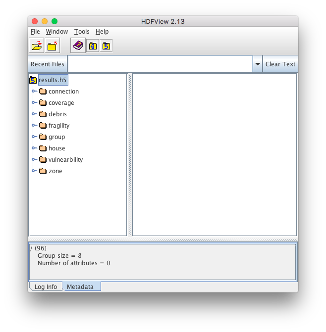
Fig. 11 Structures of output in the HDFView
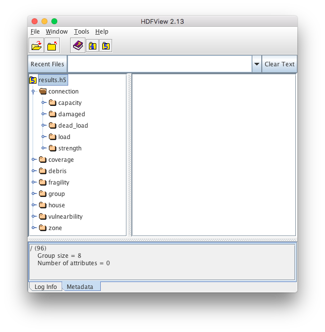
Fig. 12 Attributes under connection tab in the HDFView
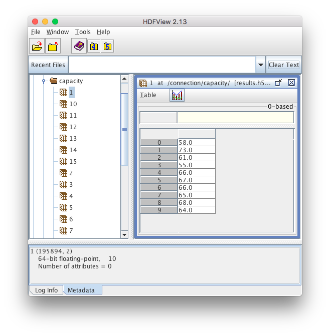
Fig. 13 Values of capacity of the selected connection in the HDFView