Workflows¶

UncoverML workflows are controlled by a YAML configuration file. This section provides some examples and explanations of different workflows, the required configuration, uncoverml commands and the produced outputs

There some example YAML files in the uncover-ml/configs directory to help you get started.

Learn and Predict¶

The most common task in UncoverML is using it train a model and then perform a prediction. This requires:

A config file with necessary parameters
A set of geotiffs containing covariate/feature data
A shapefile containing training targets

Config¶

An example of a learn/predict config:

learning:
  algorithm: transformedrandomforest
  arguments:
    n_estimators: 10
    target_transform: log

features:
  - type: ordinal
    files:
      - directory: path/to/covariates/directory
    transforms:
      - centre
      - standardise
    imputation: mean

targets:
  file: path/to/training/target/shapefile
  property: Na_log

prediction:
  quantiles: 0.95
  outbands: 4

output:
  directory: path/to/store/output

The learning block specifies the algorithm/model to train:

algorithm: the name of the algorithm
arguments: a dictionary of keyword arguments specific to that algorithm. See models page for available algorithms and links to their documentation to understand what parameters are available for each algorithm.
- target_transform: this argument is specific to UncoverML and an addition to the algorithm’s base arguments. Target values will be transformed using this method before being passed to the algorithm’s fit and predict methods.
  - identity: identity transform - does nothing to the data. This is the default option if target_transform is not provided.
  - standardise: applies a standardisation transform.
  - sqrt: applies a square root transform.
  - log: applies a log10 transform.
  - logistic: applies a logistic transform.
  - rank: apply a RankGauss transform.
  - kde: apply a KDE transform.

The features block contains the features/covariates to be used for training and prediction:

type: UncoverML supports ordinal and categorical data, but they must be provided in separate sets and the type must be provided (if no type is provided, UncoverML will assume the data is ordinal).
files: The location of the geotiffs. Multiple entries can be provided for files and can be of type directory, path or list
- directory: Path to a directory. All geotiffs within this directory will be loaded as features.
- path: Path to a geotiff file. This will be loaded as a feature.
- list: Path to a text file. Each line of the text file is a path to a geotiff and geotiff will be loaded as a feature.
transforms: Transforms to use for scaling features. Multiple transforms can be applied to each set of features specified.
- centre: applies a centre transform (demeans the data).
- standardise: applies a standardisation transform.
- log: applies a log10 transform.
- sqrt: applies a square root transform.
- whiten: applies a Whiten transform.
- onehot: performs OneHot encoding
- randomhot: performs RandomHot encoding.
imputation: the imputer to use for filling missing values in the provided features.
- mean: mean imputation.
- gauss: Gauss imputation.
- nn: nearest neighbour imputation.

Geotiffs must be the same size and resolution, otherwise an exception will be raised.

Multiple feature sets can be specified for different types of data, or for applying different transforms:

features:
  - type: categorical
    files:
      - path: path/to/categorical/feature
    transforms:
      - onehot
  - type: ordinal
    files:
      - list path/to/feature/list.txt
    transforms:
      - standardise
    imputation: nn

The targets block specifies the training targets to be used:

file: path to the shapefile containing training targets
property: name of the field in the shapefile to be used as training value. If not provided then the first field of the shapefile will be used.

At least some of the targets in the shapefile must intersect with the provided features. Targets outside of the feature area will be ignored

The prediction block specifies what outbands to generate and the quantile interval for producing upper and lower quantile maps:

quantiles: a value between 0 and 1 representing the prediction interval. E.g. ‘0.95’ means the predicted values will fall within the lower and upper quantiles 95% of the time.
outbands: each band will be written as a separate geotiff file. For classification, the available outbands is equivalent to the available classes. For regression, the first outband is prediction and if the model provides them, the next are variance, lower quantile and upper quantile. Some specific models provide further options - refer the documentation for the specific model you are using. The outbands number is used as the RHS of a slice, so providing ‘1’ for a regression will output prediction (0) and variance (1).

The output block directs UncoverML where to store learning and prediction outputs.

directory: path to a directory to store the outputs. Will be created if it does not exist. All outputs are prefixed with the config file name.

Running¶

To run this workflow, first train the model:

uncoverml learn config.yaml

Once the command is complete, outputs will exist in the directory specified in the output block.

For learning, these are:

rawcovariates.csv: a table containing the value from each covariate and the target value for a given point. This is before any scaling or transforms are applied.
rawcovariates_mask.csv: a table representing the mask for each point, i.e. which covariates are missing from which coordinates.
transformed_targets.csv: a table containing untransformed target values in the first column and the transformed value in the other column.
*.model: a Python binary file containing the trained model. It is not accessed directly but is used as part of the prediction step.

Predictions can then be performed across the entire feature space:

uncoverml predict config.yaml

Upon completion, prediction maps will be written to the output directory. There will be one map for each band requested as output in the configuration file. The map will be named after the band, e.g. prediction.tif for the main prediction band. Downsampled versions of the maps will also be generated for use as thumbnails.

Shapefile Predictions¶

Besides images, feature data can also be extracted from shapefiles. If this method is used, then the prediction will be written out as a shapefile.

Config¶

To use shapefiles, the feature block of the config must be modified:

features:
- type: ordinal
shapefile:
  file: /path/to/shapefile
  fields:
    - field1
    - field2
    - field3
  ndv: None
  transforms:
    - standardise
  imputation: mean

It’s similar to the structure for using geotiffs with some changes:

shapefile: this starts the shapefile block and signifies that shapefile training and prediction is being used. Note that currently it is not possible to mix shapefile and image features. An error will occur if you attempt to do so.
- file: path to the shapefile containing features. The file you provide must have the same number of records as your target shapefile, and must have the same geometries.
- fields: a list of fields in the shapefile that will be used as covariates.
- ndv: the no data value for the shapefile. Samples with this value will be masked out when training and predicting.

There’s also the addition of the drop parameter to the targets block:

targets:
  file: ...
  property: ...
  drop: ['unknown', 'undefined']

drop: a list of values to drop from the targets. Rows where the property field contains one of these values will be dropped when intersecting features and targets. This is for convenience of training on files with missing data that you want to predict. You can drop the rows containing the missing data for training, and then predict on the full shapefile.

Note

Currently point intersection between two shapefiles isn’t implemented. You need to ensure that your target shapefile (after any rows have been dropped) is a 1-to-1 positional match with your covariate shapefile. Both files will be ordered by position and it’s assumed they will have the same number of rows and each row in one file corresponds to a row in the other.

Running¶

Employ the same learn and predict commands as you would for learning and prediction in the learn and predict section.

The output will be the same as with image-based predictions, but instead of geotiffs, predictions will be written to a shapefile:

..._prediction.*: shapefile containing predicted values.

Model Validation¶

Validation can be performed during the training process to generate model performance metrics. UncoverML supports k-fold cross validation, out-of-sample validation, feature ranking and permutation importance.

Config¶

To perform validation, the validation block must be provided in your config file. The usual parameters for learning must be provided (see Learn and Predict).

validation:
  feature_rank: True
  permutation_importance: True
  out_of_sample:
    percentage: 0.2
    shapefile: /path/to/shapefile
    property: name_of_field
  k-fold:
    parallel: False
    folds: 5
    random_seed: 1

feature_rank: a boolean that turns feature ranking on or off.
permutation_importance: a boolean that turns permutation importance on or off.
out_of_sample: out-of-sample validation parameters
- percentage: float between 0 and 1, the percentage of targets to withhold from the training data to be used for post-learning validation.
- shapefile: path to a shapefile containing targets to be used in out-of-sample validation.
- property: name of the field in the shapefile to use as training value. If not provided then the first field of the shapefile will be used.

Note

percentage has priority over shapefile - if both are provided then the shapefile argument will be ignored.

k-fold: k-fold cross validation parameters
- parallel: a boolean that specifies whether folds are trained and predicted in parallel.
- folds: the number of folds to split training data into.
- random_seed: an integer used as the seed for the random number generator that splits folds. Using the same seed will produce deterministic fold splits.

Running¶

Model validation is performed as part of the training process. To perform model validation, run:

uncoverml learn config.yaml

Once complete, validation results will be in the output directory:

crossval_results.csv: A table of target values and corresponding predicted value for k-fold.
crossval_scores.json: A dictionary containing the value for each metric for k-fold.
featureranks.json: Dictionaries containing feature rank results. The ranks dictionary presents the most important feature by its impact on each metric (which feature caused the most degradation of the metric when excluded from training). The scores dictionary contains the corresponding value for each rank.
permutation_importance.csv: The permutation importance results.
oos_results.csv: A table of targets values and corresponding predicted value for out-of-sample validation.
oos_scores.json: A dictionary containing the value for each metric for out-of-sample validation.
oos_targets.shp: If percentage was provided as part of out-of-sample arguments, the withheld targets will be saved to this shapefile for reuse.

In addition to these, the ‘prediction’ column of rawcovariates.csv will be filled with the corresponding prediction value generated during cross-validation.

Diagnostics¶

UncoverML can generate diagnostic plots. These are controlled by additional parameters in the output block:

output:
  directory: path/to/output/directory
  plot_feature_ranks: True
  plot_intersection: True
  plot_real_vs_pred: True
  plot_correlation: True
  plot_target_scaling: True

Covariate Correlation¶

This generates a correlation matrix showing correlation between provided covariates. The color/value of each square shows how strong the positive or negative correlation is:

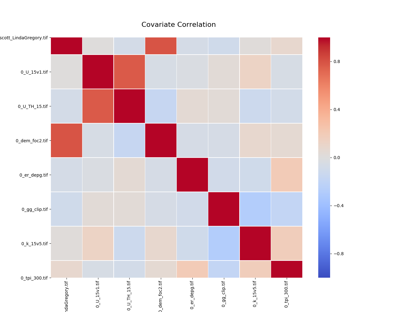
To generate a correlation matrix, the learn command must be run with plot_correlation set to True in the configuration.

Feature Ranking¶

The result of feature ranking can be plotted. This creates two plots. One is a grouped bar chart - each colored bar represents a metric, the Y-axis is the score of that metric and each group is a feature (AKA covariate):

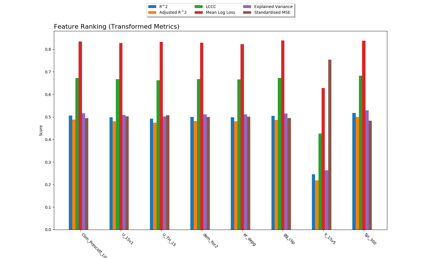
_images/sirsam_Na_randomforest_featureranks.png

The other plot is a series of curves. Each curve represents a metric, with scores on the Y-axis and covariates on the X-axis. Each inflection represents what happens to the score when the corresponding covariate is removed from the model:

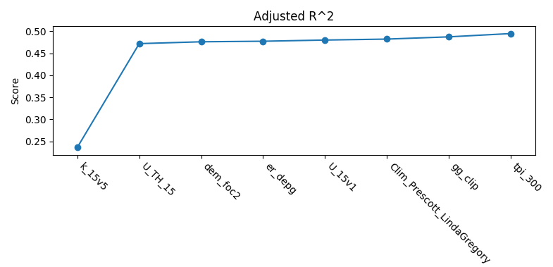
To generate feature rank plots, the learn command must be run with feature_rank set to True under the validation block of the config, and plot_feature_ranks set to True.

Covariate Intersection¶

Covariate intersection can be plotted. These scatter plots, one for each covariate, show the corresponding covariate value for each target value:

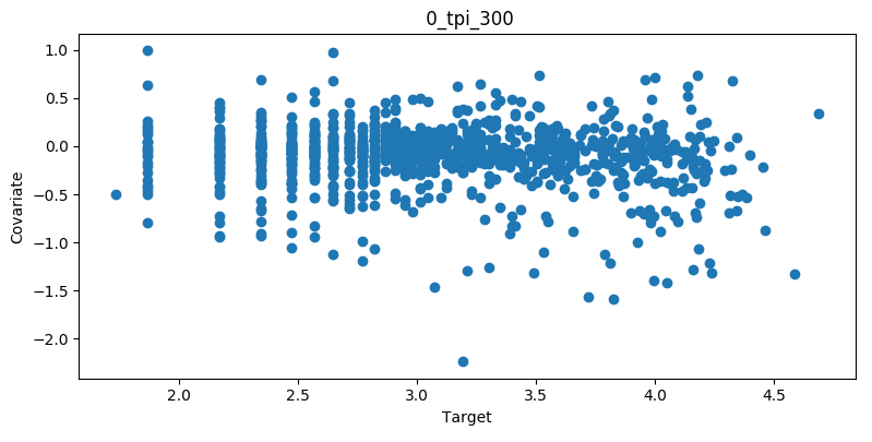
To generate intersection plots, the learn command must be run and plot_intersection must be True in the configuration.

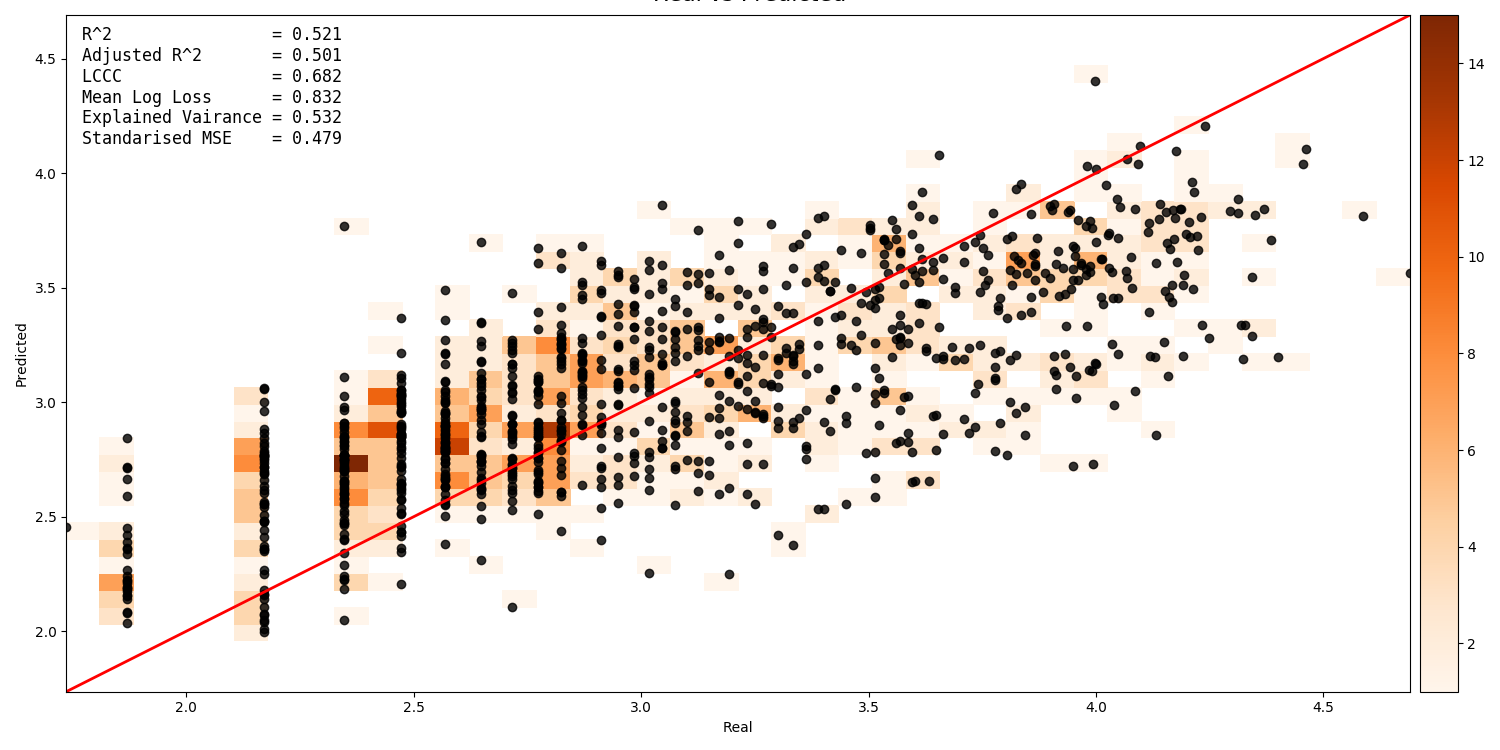
Real vs. Prediction¶

A scatter plot showing the intersection between real vs. predicted values can be generated. This compares the values predicted by the model to the actual target values, and is important for validating model. It includes several pieces of information. The points show the intersecting values. The 2D histogram in the background shows grouping of the points (the colorbar on the right-hand side codes the frequency of each grouping). The text in the upper-left shows the score from the metrics generated by cross-validation:

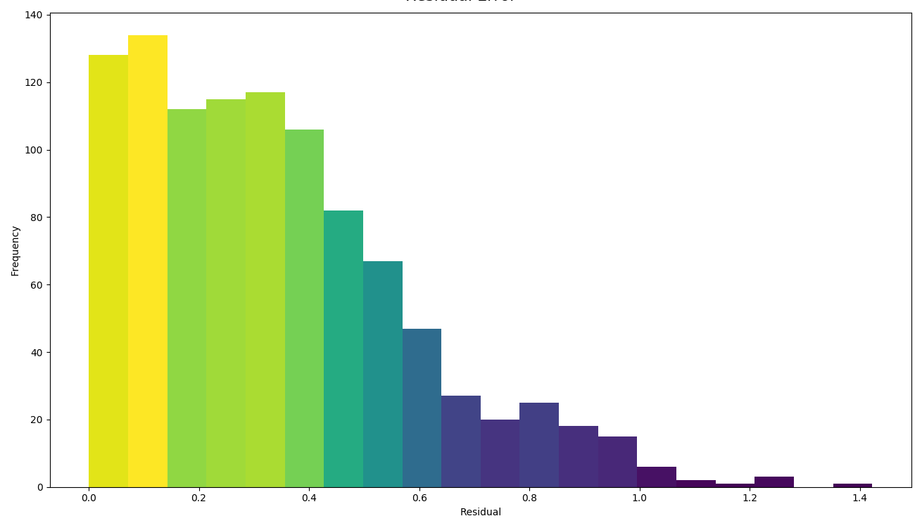
_images/sirsam_Na_randomforest_real_vs_pred.png

A histogram of residual error is also generated. This shows bins grouping the residual error between intersected points (i.e. the difference between a predicted value and the corresponding real value):

_images/sirsam_Na_randomforest_residual.png

To generate a real vs. prediction plot, k-fold must be enabled under the validation block of the config, and plot_real_vs_pred must be set to True.

Multiprocessing and Partitioning¶

UncoverML supports parallelization using MPI and also supports partitioning for large datasets. When and how to use these depends on the task being performed.

Learning¶

When running learn, it can be beneficial to use multiple processors to train folds for k-fold cross validation in parallel. For example, if you have enabled crossval with 5 folds and set parallel: True in the k-fold block, then you can train the folds in parallel using:

mpirun -n 5 uncoverml learn config.yaml

This will speed up the cross-validation process.

If not utilising parallel crossval, there is no benefit to using multiple processors. A model can only be trained on a single processor, so to avoid wasting compute resources, train models with 1 processor:

uncoverml learn config.yaml
# equivalent to `mpirun -n 1 uncoverml learn config.yaml`

An exception is when learning an ensemble model. Examples are bootstrapsvr and multirandomforest. These are ensembles of several individual models. When training an ensemble model, it can be beneficial to run with multiple processors as each processor can train a submodel. Note that running with more processors than there are submodels to train will waste compute resources as the remainder (n_processors - n_models) processors will have no work to perform.

For example, if you were training a bootstrapsvr model with 100 models, and you were running on a single HPC node with 48 cpus, you can run in parallel using:

mpirun -n 48 uncoverml learn config.yaml

This will greatly reduce the training time of an ensemble model.

Prediction¶

Prediction gains the most benefits from multiprocessing and partitioning. Because the model is already trained, prediction can be done by splitting up the feature space into chunks and distributing them to processors to speed up prediction. These chunks can then also be further partitioned and loaded sequentially on each processor to reduce memory usage.

While multiple CPUs will speed up prediction, partitioning will have an impact on speed, as it increases I/O overhead. However, it allows prediction on larger-than-memory datasets.

For example:

mpirun -n 48 uncoverml predict config.yaml -p 5

This command will split the feature data into 48 even chunks and distribute it amongst the CPUs. Each chunk will then be split into 5 partitions (the -p 5 parameter) and loaded, predicted on and written out sequentially, reducing memory usage.

Optimisation¶

UncoverML provides a framework for using scikit-learn’s GridSearchCV to perform hyperparameter tuning. This allows cross-validation to be performed with different combinations of parameters.

Note

Only some models are compatible with optimisation. This is because models must be structured in a way compatible with scikit-learn’s GridSearchCV. This involves:

having all arguments explicitly listed in the __init__ signature (no varargs)
having the expected functions (fit, predict, etc.)
implementing the get_params and set_params functions defined by Base Estimator

Optimisable models are listed in the models section.

Config¶

An example config for performing optimisation on transformedrandomforest:

optimisation:
  algorithm: transformedrandomforest
  scorers: [r2, expvar, smse, lins_ccc]
  hyperparameters:
      target_transform: [identity, standardise, log, sqrt]
      n_estimator: [10, 20, 50]
      max_features: [auto, sqrt, log2]
      min_samples_split: [2, 5, 10]
      min_samples_leaf: [1, 5, 10]
      max_depth: [10, 20, 100]

output:
    directory: path/to/output/directory

algorithm: name of the algorithm to optimise.
scorers: a list of metrics to consider when ranking parameter combinations.
- r2, expvar, smse and lins_ccc are the available regression model parameters.
- accuracy, log_loss and auc are applicable to classifiers.
hyperparameters: contains lists of values for various algorithm parameters - view the documentation for the algorithm to know parameters are available. Every permutation of the given parameters will be scored using cross-validation.

Running¶

Optimisation is run using:

uncoverml gridsearch config.yaml -n 10

The -n 10 is the number of parallel workers to use. Gridsearch uses the joblib backend, so don’t use mpirun to execute it, but rather set -n to the number of processors you have available.

The output will be in the output directory:

optimisation.csv: a table of gridsearch results. For details, see the documentation for cv_results_ attribute in the sklearn docs.

Shiftmap¶

UncoverML has a shiftmap feature that generates a map of the covariate shift in your feature space. ‘Covariate shift’ is the shifting of covariate distributions across different areas.

The idea behind shiftmap is to generate ‘dummy’ targets, equal in number to the provided training targets. These dummy targets are distributed randomly across the feature space.

The two sets of targets (dummy and real) are labeled ‘query’ and ‘training’ respectively. A logistic classifier is then trained on these targets and classification maps are generated.

Areas where the classifier can’t distinguish between the two classes (e.g. 0.4 - 0.6 certainty for one or the other class) means the covariate data in that area has a similar distribution to the provided training data. In theory, these are areas where the model can be extrapolated and will perform well, as the distribution is similar to the provided training data. Areas with a strong covariate shift (e.g. 0 - 0.4, 0.6 - 1 certainty for either class) may not be suitable for extrapolating the model due to differences in distribution between training data and feature data.

Running¶

Shiftmap requires a standard learning config and doesn’t require extra parameters. To run:

uncoverml shiftmap config.yaml

Covariate shiftmaps will be written to the output directory:

shiftmap_generated_points.csv: a table of the randomly generated points which can be used for validation and debugging.
shiftmap_query_0.tif: a map showing the likelihood of each pixel belonging to the ‘query’ class. Areas of uncertainty (0.4 - 0.6 for example) are areas with similar distributions to the training data.
shiftmap_training_1.tif: same as above but inverted; shows the likelihood of each pixel belonging to the training class.
most_likely.tif: a map showing which class each pixel is most likely to belong. This can be ignored as it does not help demonstrate the covariate shift, but is left for debugging purposes.

Target Search¶

UncoverML implements a novel targetsearch command. Targetsearch is used to help find subsets of training points that are similar to a particular study area.

For example, you might have a national dataset of geochem points and you want to predict the potassium content for a much smaller study area. Instead of supplying the entire geochem dataset, you can use target search to determine which points in the dataset are most similar to the study area (i.e. which points have a similar distribution of feature data) and these are the points are used in addition to the provided training targets for training the model.

Config¶

Target searching is performed by adding parameters to the learning block of the config:

learning:
  target_search: True
  target_search_threshold: 0.8
  target_search_extents:
    xmin: 120
    ymin: -20
    xmax: 121
    ymax: -21
  algorithm: transformedrandomforest
  arguments:
    n_estimators: 10
    target_transform: log

target_search: a boolean of whether or not to use targetsearch
target_search_threshold: the likelihood threshold a training point must surpass to be included in found points (i.e. how similar a training points feature distribution is to the study area)
target_search_extents: extents defining the study area. Target search will select points from the training targets that have a similar feature distribution to this study area.

Running¶

To select and return the targets, first run targetsearch:

uncoverml targetsearch config.yaml

In the output directory, there are three files:

targetsearch_generated_points.csv: a list of points that were randomly generated in the study area, used for validation and debugging.
targetsearch_likelihood: the likelihood of each training target belonging to the study area
targetsearch_result.pk: a Python binary file containing the training targets that have surpassed the target_search_threshold.

Once the targets have been selected, they can be used in training a model by passing the same config to the learn command:

uncoverml learn config.yaml

Learning will run as normal, with the addition that the targets selected by target_search will be included with the provided training targets and used to train the model.

Cropping¶

UncoverML has a built-in cropping function that is useful for a variety of purposes. By providing a bounding box of xmin, xmax, ymin, ymax, all geotiffs provided to the uncoverml command will be cropped to this extent before processing takes place.

Original files will be maintained and the cropped versions are stored temporarily then removed by UncoverML on completion.

Config¶

Cropping is performed by providing the extents block in the config:

extents:
  pixel_coordinates: False
  xmin: 120
  ymin: -20
  xmax: 121
  ymax: -21

pixel_coordinates: boolean indicating whether to treat the given crop coordinates as pixels (True) or as coordinates in the CRS used by the covariate geotiffs (False). If using pixel coordinates, these start at 0 and extend to the width and height of the image, inclusive.
xmin, ymin, xmax, ymax: coordinates of the crop box. If not provided or out of bounds of the covariate images, then the default bound of the covariate bounds is used respectively.

Running¶

Cropping applies to the learn, predict, shiftmap and targetsearch commands of UncoverML.

Running learn with the above extents in the config will crop the provided covariates to that extent, and the model will be trained on the remaining data. Similarly, running prediction with the extents block will crop the covariates and only predict on the remaining data.

This is very useful for speeding up jobs or in situations where the data is too large for memory. It’s also convenient when providing covariates of different sizes. UncoverML doesn’t support this, but by setting the extents as the smallest intersecting area of the covariates, an intersecting stack of feature data can be generated and used for training and prediction.

Using cropping to perform parallel predictions¶

Another use is for running parallel prediction jobs. For large-scale jobs, particularly when using ensemble models and on HPC platforms, it can be beneficial to break up prediction into multiple jobs and launch them in parallel.

To achieve this, first train the model on your full dataset. Then create multiple prediction configs, each one predicting on a chunk of the data:

extents:
  pixel_coordinates: True
  xmin: 0
  ymin: 0
  xmax: 1000
  ymax: 1000

output:
  directory: path/to/output/directory

Repeat this, providing the extents for each chunk until the whole dataset is covered. Once you have chunk1.yaml, chunk2.yaml etc., submit them as individual prediction jobs:

uncoverml predict chunk1.yaml

Doing so for each chunk config.

Upon completion you will have multiple prediction maps prefixed with the config name, e.g. chunk1_prediction.tif. Using a GIS viewer or other program, you can then stitch the prediction chunks together.

Clustering¶

UncoverML supports k-means clustering.

Config¶

When providing a clustering block, learning, validation and targets blocks don’t apply and are not required. features must be provided for training and prediction and prediction block for predicting the k-means model.

clustering:
  file: /path/to/class_labels.shp
  property: name_of_class_label_property
  n_classes: 5
  oversample_factor: 5

file: path to shapefile containing labels. This is optional. If provided then semi-supervised clustering is performed, other clustering is unsupervised.
property: the name of the class label property in the shapefile. Only required if a shapefile has been provided and semi-supervised clustering is being performed.
n_classes: the number of classes to cluster the data into.
oversample_factor: controls the number of samples drawn as part of the initialisation step. More processors used will increase the total number of samples drawn. Consider values of 1 for more than 16 processors.

Running¶

uncoverml cluster config.yaml

will train and output the k-means model file.

uncoverml predict config.yaml

will produce a map showing which pixel each class is most likely to belong to.

Weighted Samples¶

Some models support a sample_weight parameter. Look at the documentation of the fit method for the selected algorithm to see if this is available.

Sample weights can be provided by creating a weight field in your target shapefile. Weights are integer values that signify the relative importance of a sample. Weights of 0 mean the sample will be excluded entirely.

Config¶

Weights are applied by providing the name of the weight field to the targets block.

targets:
  file: path/to/targets/shapefile.shp
  property: training_field
  weight_property: weight_field

Running¶

Run learning as normal:

uncoverml learn config.yaml

There will be a log info message stating ‘Sample weights are being provided to fit method’ when the model is trained. If the model does not support sample weights, then there will be a log info message ‘Model does not support sample weights, weights are being ignored’ and unweighted training will continue.

Prediction Mask¶

A crop mask can be provided when performing predictions. This mask will cause prediction to only predict and write values that have a certain mask value. This is useful for masking out no data areas such as the ocean, or limiting predictions to an area of interest to increase performance.

The geotiff must be the same size as the provided covariates. Cropping also applies to prediction masks.

Config¶

To supply a mask, add the mask block to your config:

mask:
  file: path/to/mask.tif
  retain: 1

file: path to the mask geotiff
retain: value in the mask denoting which pixels to predict

Running¶

Run prediction as normal:

uncoverml predict config.yaml

Adding fields to output table¶

Any field in the target shapefile can be written to the rawcovariates.csv output table. This can be helpful for validation and debugging, e.g. including the type or category of the sample in the results.

Config¶

To include fields in the output table, add the write_to_csv parameter to your targets block:

targets:
  file: path/to/targets/shapefile.shp
  property: training_field
  write_to_csv: [type, site_id]

write_to_csv: list of names of shapefile fields to include in the rawcovariates.csv output table.

Running¶

Run learn as normal and the fields will be included in the output table:

uncoverml learn config.yaml

Resampling¶

UncoverML has a resample tool that allows a target shapefile to be resampled based on value or spatial parameters.

Config¶

Resampling requires a targets block with additional resampling parameters and an output block specifying a directory.

targets:
  file: path/to/targets/shapefile
  property: target_field_name
  resample:
    spatial:
      rows: 10
      cols: 10
      bootstrap: False
      output_samples: 1000
      fields_to_keep: [type, site_id]
    value:
      bins: 3
      bootstrap: True
      interval: linear
      fields_to_keep: [type, site_id]

output:
  directory: ./resampling_out

file: path to the target shapefile
property: name of the target observation field
resample: the resampling arguments
- spatial: arguments for spatial resampling - rows, cols: int, the number of rows and columns to divide
  
  the shapefile area into. Each resulting cell is a bin.
  - bootstrap: boolean, whether to sample with replacement. If true, then duplicate samples are allowed, otherwise each value will only be sampled once at most.
  - output_samples: int, the number of output samples. This is the total number, so the number of samples in each bin is equal to (output_samples // bins)). If bootstrap is false and there are not enough samples in a bin to fulfill the requested number, then all samples will be taken and the bin will be short of samples.
  - fields_to_keep: by default, the only value preserved in the resulting resampled shapefile is the property specified by property. To keep additional fields, add them to this parameter.
- value: arguments for value resampling - bins: the number of bins to divide samples into. - interval: linear or percentile, the method for
  
  determining bin edges. If linear then bin edges will be taken at equally spaced intervals from the min to the max of the target values.
  
  E.g., if bins is 3 and the data range is 0 to 300, then the bins will be 0 to 100, 100 to 200 and 200 to 300.
  
  If percentile then the bin edges will be the Nth percentile value of the target data, with the percentiles being the result of linearly spacing the number of bin edges between 0 to 1.
  
  E.g., if bins is 3, then the bins will cover from 0 to 33rd percentile, 33rd to 66th percentile and 66th to 100th percentile.

Running¶

To perform resampling, run:

uncoverml resample config.yaml

Output will be in the output directory, with the resampled shapefile in a subdirectory having the original shapefile name appended with ‘resampled’.

Covariate Diagnostics¶

UncoverML includes a covdiag command for convenience. This will output some basic diagnostics for your covariates.

Running¶

Covdiag can be run on a single covariate:

uncoverml covdiag path/to/tif

Or on a directory. Adding -r flag will explore the directory recursively, outputting diagnostics for all tiffs in all subdirectories.

uncoverml covdiag path/to/covariate/directory -r

By default, output is delivered to the console. To save to a textfile, use output redirection:

uncoverml covdiag /path/to/covariate/directory >> output.txt